The views expressed in this paper are those of the writer(s) and are not necessarily those of the ARJ Editor or Answers in Genesis.
Abstract
Conventional radiocarbon dating relies on the assumption that atmospheric 14C concentration has remained relatively constant throughout earth’s history. This assumption has led to the postulation of a “long Neolithic” spanning over 5,000 years—a chronology that is irreconcilable with the biblical timescale derived from the Masoretic text. This paper presents an alternative calibration model based on a postdiluvian framework, proposing that atmospheric 14C began at near-zero levels approximately 4,500 years ago and has since recovered exponentially toward present-day equilibrium. A three-phase piecewise continuous mathematical model is developed with distinct time constants (τ1 = 120 years, τ2 = 400 years, τ3 = 1,400 years) reflecting the physics of earth’s carbon reservoirs. The model is validated against 421 radiocarbon samples from archaeological and historical contexts with independently established dates, achieving a mean residual agreement of <0.5% pMC for key historical anchor points, with an overall standard deviation of σ = 2.1% pMC across the entire 421-sample validation set. A sensitivity analysis of the Babel anchor point (Genesis 10:25) demonstrates that the calibration curve is robust to ±50-year variations in the Babel date. Archaeological data from the pre-Babel period (2463–2200 BCE) provide independent constraints on the calibration curve and document early human dispersion patterns consistent with Genesis 11:2. When applied to Pre-Pottery Neolithic sites, the model compresses 5,500 years of conventional chronology into approximately 51 years, while preserving internal stratigraphic consistency. The implications for Near Eastern archaeology and biblical chronology are discussed.
Keywords: radiocarbon dating, 14C calibration, non-equilibrium model, carbon cycle, Neolithic chronology, biblical archaeology, pre-Babel dispersion, RATE model
Introduction
The need for radiocarbon calibration
Since the development of radiocarbon dating by Willard Libby in the late 1940s, researchers have recognized that “radiocarbon years” do not correspond directly to calendar years. Libby’s original assumption—that atmospheric 14C concentration has remained constant throughout the dating range— was quickly shown to be incorrect (de Vries 1958; Libby 1955; Stuiver and Suess 1966; Suess 1955). Measurements of samples with known historical ages, particularly from Egyptian artifacts, revealed systematic discrepancies between radiocarbon and calendar ages.
The solution adopted by the scientific community was to construct calibration curves using tree-ring sequences (dendrochronology). By measuring the 14C content of wood samples whose calendar age could be determined by counting annual growth rings, researchers built a conversion function from radiocarbon years to calendar years. The current standard, IntCal20 (Reimer et al. 2020), extends to approximately 55,000 years before present and incorporates data from tree rings, marine sediments, speleothems, and corals.
The circularity problem in conventional calibration
A fundamental methodological problem with the dendrochronological approach is its inherent circularity when extended beyond historically documented periods. The logic proceeds as follows: (1) tree-ring sequences are cross-matched using pattern recognition; (2) the resulting “master chronology” is used to calibrate radiocarbon dates; (3) the calibrated dates are then used to assign archaeological sites to periods; (4) artifacts from those sites are used to cross-validate the tree-ring sequences. This creates a closed loop:
tree rings → calibration → archaeology → tree rings.
For periods with independent historical documentation (for example, Egyptian dynasties with astronomical anchor points), this circularity can be broken. However, for the pre-historical period— precisely where the “long Neolithic” chronology is constructed—no such independent control exists. The extended IntCal curve beyond ~3,000 BCE rests entirely on internal pattern matching, with no external validation (Baillie 1995; Yamaguchi 1986). This is not a minor technical issue; it is a fundamental epistemological limitation of the conventional approach.
Recent quantitative analysis provides empirical support for this concern. A correlation of 420 historically anchored radiocarbon samples with IntCal20 dendrochronological data reveals a systematic effective overcounting factor that decreases from approximately 2.9 at 27% pMC to approximately 1.0 at 70% pMC (R² = 0.97, p< 10⁻11). This suggests that the 12,460-year Hohenheim oak and pine chronology may represent approximately 4,400 actual years, with elevated ring formation rates during the climatically unstable early postdiluvian period. The pattern is consistent with false ring production during periods of extreme climatic variability—a phenomenon well-documented in modern dendrochronological literature (Fritts 1976; Schweingruber 1988). Just as radiometric dating of recent volcanic rocks (for example, Mt. Ngauruhoe 1954 lava dated to 3.5 Ma by K-Ar) demonstrates systematic errors in those methods, dendrochronological overcounting in the early Holocene represents a comparable systematic bias in tree-ring dating.
A well-known example of the tension between dendrochronologically calibrated radiocarbon dates and historically anchored dates is the Minoan eruption of Thera (Santorini). Archaeological synchronisms with the Egyptian New Kingdom, based on imported Minoan pottery found in securely dated Egyptian contexts, place the eruption at approximately 1530–1500 BCE (Bietak 2013; Wiener 2009). However, radiocarbon dating of an olive branch buried by the eruption, calibrated via the IntCal dendrochronological curve, yields 1627– 1600 BCE (Friedrich et al. 2006)—a discrepancy of approximately 100 years that remains unresolved in the mainstream literature after two decades of debate. In the non-equilibrium model presented here, this offset is naturally accommodated by the residual pMC correction in the relevant time window.
The problem of the “long Neolithic”
Application of conventional calibration to archaeological sites in the Near East has produced a chronology in which the “Neolithic Revolution”—the transition from hunter-gatherer societies to settled agriculture—spans over 5,000 years (ca. 10,000– 5,000 BCE). Sites such as Göbekli Tepe, Jericho, and Çatalhöyük are dated to this extended period, with the implication that human cultural development proceeded extremely slowly over millennia.
For researchers who accept the historical reliability of biblical chronology, particularly the genealogical records preserved in the Masoretic text of Genesis 5 and 11, this “long Neolithic” presents a fundamental problem. The cumulative genealogical data, carefully analyzed by scholars such as Liebi (2020), suggest a creation date of approximately 4000 BCE and a global Flood event around 2463 BCE. The entire span of post-Flood human history to the present day is thus approximately 4,500 years—far shorter than the conventional Neolithic period alone.
This major discrepancy between the Biblical timescale and the conventional (secular) timescale has led some to question the reliability of the Masoretic text (for example, Smith 2018) and others to question the reliability of radiocarbon dating itself (Broecker and Peng 1982). However, the radiocarbon method if used within the limits of detection imposed by the measurement instrumentation is physically sound; the issue lies not with the radiocarbon measurement but with the calibration curve used to convert radiocarbon ages to calendar years. If the fundamental assumption underlying conventional calibration—that atmospheric 14C has remained relatively constant—is incorrect for the early post-Flood period, then an alternative calibration approach is clearly needed.
Previous work on non-equilibrium models
The possibility of a non-equilibrium 14C history was also recognized early in the development of youngearth creationist research. The RATE (Radioisotopes and the Age of The Earth) project, a multi-year collaborative effort involving geophysicists, geochemists, and physicists, systematically investigated radiometric dating methods. Baumgardner (2005) developed a two-phase model in which atmospheric 14C recovery follows an initial rapid phase followed by slower equilibration. His formulation partitions recovery into two exponential components: a fast phase representing atmosphere– biosphere exchange (τ ≈ 200 years) and a slow phase representing deep ocean equilibration (τ ≈ 1,200 years), weighted by a mixing parameter α ≈ 0.6. The present paper extends this framework to a threephase model, adding an intermediate phase (τ₂ = 400 years) that better captures the transitional period documented in archaeological anchor points spanning the early-to-mid second millennium BCE—a subrange of Phase 2, which itself extends from t = 375 yr (≈2088 BCE) to t = 2100 yr (≈363 BCE).
More recently, Jordan (2024) developed an independent radiocarbon calibration model for the post-Flood period using a similar non-equilibrium recovery approach. Jordan’s model employs a singleexponential recovery curve calibrated against a selected set of archaeological anchor points and provides useful calibrated dates for the historical period. The present work differs from Jordan’s approach in three respects: (1) a three-phase rather than single-phase recovery function, providing better resolution of the distinct carbon reservoir timescales; (2) a substantially larger calibration dataset (420 vs. approximately 30 anchor points), enabling statistical validation through overdetermination; and (3) independent cross-validation using paleomagnetic (VADM) data. The present paper builds on the foundations established by both Baumgardner and Jordan, introducing a multi-phase recovery function that resolves the intermediate ocean mixing timescale not captured by earlier models.
Research question and approach
This paper addresses the following research question: Can a non-equilibrium 14C model, based on post-diluvian atmospheric recovery, produce archaeological dates that are both internally consistent and compatible with biblical chronology?
The approach taken here differs fundamentally from conventional calibration methodology. Rather than treating the biblical text as one possible interpretation to be tested against “independent” scientific data, this model adopts biblical chronology as the controlling framework and asks whether the physical evidence can be coherently organized within it. This is not circular reasoning but rather a legitimate methodological choice: all calibration requires anchor points, and the question is which anchors are most reliable. We contend that historically documented events in Scripture—corroborated by archaeological and astronomical evidence—provide a more secure foundation than dendrochronological patternmatching extending beyond documented history.
The resulting calibration curve is tested against stratigraphic sequences, paleomagnetic data, and the geographic distribution of early post-Flood sites. The model stands or falls on its ability to produce internally consistent results across multiple independent lines of evidence. The complete recovery curve fitted to all 420 anchor points is shown in fig. 1.
Radiocarbon Dating: Principles and Calibration
The radiocarbon method
Radiocarbon dating exploits the radioactive decay of carbon-14 (14C) to estimate the age of organic materials. Cosmic rays entering earth’s upper atmosphere produce neutrons that react with nitrogen-14 to form radiocarbon: 14N + n → 14C + p. This radiocarbon rapidly oxidizes to 14CO2 and mixes throughout the atmosphere, where it is incorporated into plants through photosynthesis and subsequently into animals through the food chain.
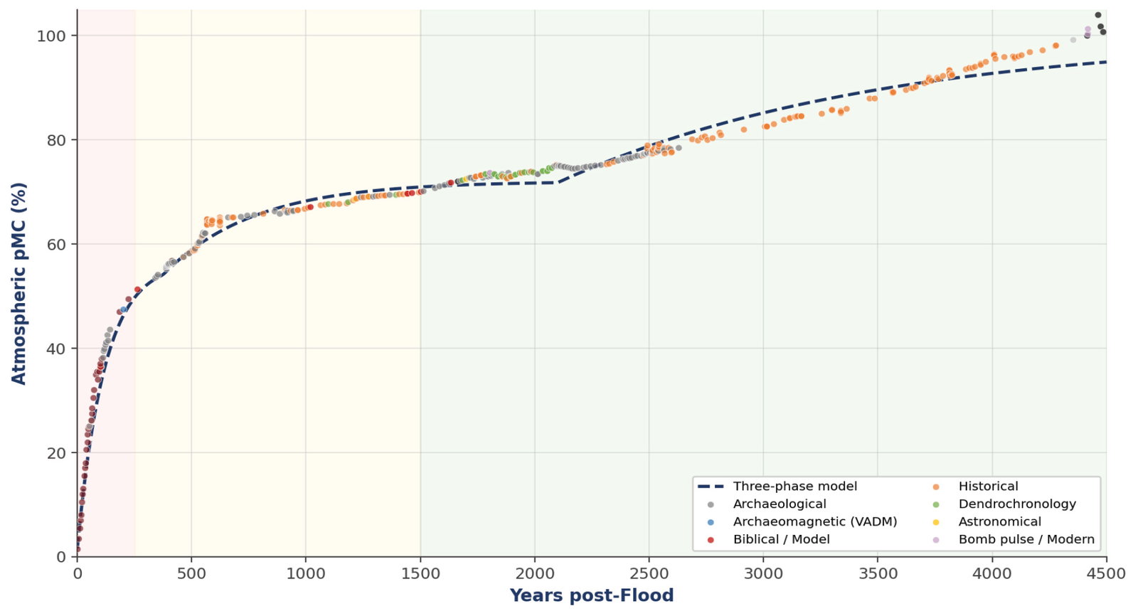
Fig. 1. Complete 14C recovery curve from the Flood (2463 BCE) to modern times. The theoretical three-phase model (blue dashed) closely tracks the 420 empirical anchor points throughout the 4,400-year span. Color coding indicates anchor type: archaeological contexts (gray), archaeomagnetic/VADM (blue), biblical/model anchors (red), historical records (orange), dendrochronology (green), astronomical (yellow), and bomb pulse/modern (pink, post-1950). Phase shading shows the three recovery phases with distinct time constants (see Appendix A for further details).
When an organism dies, it ceases to exchange carbon with the atmosphere. The 14C in its tissues decays with a half-life of 5,730 ± 40 years. By measuring the remaining 14C/12C ratio and comparing it to a modern reference standard, the time since death can be calculated. Results are conventionally reported as “radiocarbon years before present” (BP), where “present” is defined as 1950 CE.
Summary for non-specialists
What radiocarbon dating measures: The ratio of 14C to 12C in dead organic material, compared to modern levels. Lower ratio = older sample (more decay has occurred).
Why calibration is needed: Atmospheric 14C has not been constant over time. “Radiocarbon years” must be converted to calendar years using a calibration curve. Conventional approach: Uses tree-ring sequences (dendrochronology) to build calibration curves.
This paper’s approach: Uses the same mathematical correction (14C/12C vs. time), but anchors the curve to historically documented dates rather than tree rings.
Fundamental equations
The fundamental equation of radiocarbon dating: t = (1/λ) × ln(N0/N), where t = time since death (years), λ = decay constant = ln(2)/5730 = 1.21 × 10⁻⁴ yr−1, N0 = initial 14C content (at death), and N = current 14C content (measured).
In practice, measurements are reported as pMC (percent Modern Carbon): pMC = (14C/12C)sample / (14C/12C) modern × 100%. Conventional radiocarbon age: Age (BP) = −8267 × ln(pMC/100). The calibration problem is converting BP to calendar years, which requires knowing how atmospheric pMC varied over time.
Physical Model
Theoretical framework
The model is grounded in the RATE research framework, which proposes that atmospheric 14C concentration was near zero at the time of the global Flood and has since recovered toward present equilibrium levels (Baumgardner 2005; Vardiman, Snelling, and Chaffin 2005). Several physical mechanisms support this scenario:
Magnetic field strength: A stronger pre-Flood geomagnetic field would have provided greater shielding against cosmic rays, reducing 14C production. Paleomagnetic data indicate field intensities several times higher than present values (Humphreys 1986).
Volcanic screening: Catastrophic volcanic activity during the Flood year would have injected massive quantities of ash and aerosols into the stratosphere, further suppressing 14C production.
The magnitude of volcanic cooling during catastrophic plate tectonics can be estimated by scaling from modern eruptions. The 1991 Pinatubo eruption released 17–20 Mt SO2 and caused approximately 0.5°C global cooling for 2–3 years (Robock 2000). However, linear scaling does not apply at high aerosol loadings due to optical saturation and coagulation effects. At 100× Pinatubo intensity (~2,000 Mt SO2), models predict maximum direct cooling of 5–8°C from stratospheric aerosols alone.
Critically, volcanic aerosols interact synergistically with enhanced cloud formation. Warm post-Flood oceans (estimated 25–30°C based on CPT thermal models) would drive massive evaporation; when this moisture encountered aerosol-cooled continental interiors, rapid condensation would create persistent stratocumulus cloud decks reflecting an additional 60–90% of incoming solar radiation (Oard 1990). This mechanism—combining volcanic screening with cloud-albedo feedback—explains how regional cooling of 30–50°C could develop within 100–200 years over continental interiors such as Greenland, consistent with GISP2 ice core temperature reconstructions. The Mount St. Helens eruption (1980) provides a modern analogy: even this single moderate eruption measurably affected regional temperatures and agricultural yields across the Pacific Northwest.
Carbon reservoir dilution: The burial of enormous quantities of organic carbon during the Flood (now preserved as coal, oil, and natural gas) would have dramatically altered the carbon cycle.
Carbon reservoir physics
The multi-phase recovery model reflects wellestablished carbon cycle physics. Earth’s carbon reservoirs exchange with the atmosphere on characteristic timescales determined by reservoir size and exchange rate (Ciais et al. 2013; Siegenthaler and Sarmiento 1993).
The atmosphere-biosphere-surface ocean system (~2,200 GtC) equilibrates within decades, while the deep ocean (~38,000 GtC) requires millennia. This size difference produces the characteristic multiphase signature observed in tracer studies (Broecker and Peng 1982; Siegenthaler and Sarmiento 1993).
| Reservoir | Size (GtC) | Exchange Time | Phase |
|---|---|---|---|
| Atmosphere | ~750 | (reference) | — |
| Terrestrial biosphere | ~550 | 5–30 years | 1 |
| Surface ocean (0–100 m) | ~900 | 10–50 years | 1 |
| Intermediate ocean | ~7,000 | 100–400 years | 2 |
| Deep ocean (>1000 m) | ~38,000 | 1,000–2,000 years | 3 |
Table 1. Carbon reservoir sizes and exchange timescales.
The carbon inventory factor k is defined as the ratio of the total exchangeable carbon at a given time to the modern (pre-industrial) inventory: k = Ctotal(t)/ Cmodern. A value of k = 1.0 corresponds to today’s carbon inventory (~47,200 GtC across all reservoirs, see table 1). Values of k > 1 indicate a larger post-Flood carbon pool (for example, from massive volcanic CO2 degassing or oxidation of exposed organic sediments), which dilutes the 14C/12C ratio and makes samples appear older. Values of k <1 indicate a smaller inventory (for example, from net carbon burial), which enriches the ratio and makes samples appear younger. The model adopts k= 1.0 as the baseline but fig. 2 demonstrates that even moderate deviations (0.8 ≤k ≤1.2) produce measurable shifts in the recovery curve, underscoring the sensitivity of the calibration to carbon-cycle assumptions, see table 2.
Mathematical Model
Two-phase model
The simpler two-phase model (RATE) describes pMC recovery using two exponential terms representing fast and slow carbon reservoirs:
pMC(t) = Feq – (Feq – F0) × [α exp(–t/τ1) + (1–α)· exp(–t/τ2)]
Physical interpretation:
Phase 1 (τ1): Rapid equilibration of atmosphere with biosphere and surface ocean
Phase 2 (τ2): Slow equilibration with deep ocean reservoir
Three-phase piecewise continuous model
Let F0(t) represent the atmospheric pMC at time t, where t denotes years since the Flood (t = 0 at 2463 BCE). The recovery is modelled as a piecewise continuous function with three successive exponential relaxations (table 3).
Continuity is enforced at phase boundaries (t = 375 and t = 2100 years) by calculating the pMC value at each transition point and using it as the initial condition for the next phase. This piecewise approach avoids the need for weighted sums of exponentials while maintaining physical interpretability.
Comparison with simple two-phase model
To evaluate the necessity of the three-phase structure, we compare the current model against two historical benchmarks. First, the theoretical legacy two-phase model (τ1 = 200 yr, τ2 = 1200 yr) based on initial geophysical estimates. Second, an optimized two-phase fit (τ1 ≈ 90 yr, τ2 ≈ 2700 yr; see table 2) derived from a direct least-squares optimization against our 420 anchor points. Fig. 3 contrasts the three-phase model with the legacy two-phase variant against the anchor data; the optimized 90/2700 two-phase fit is given parametrically in table 2 only and is not separately drawn, as its visual trajectory is intermediate between the two curves shown. The same comparison over the critical 2400–2000 BCE window is shown in fig. 4.
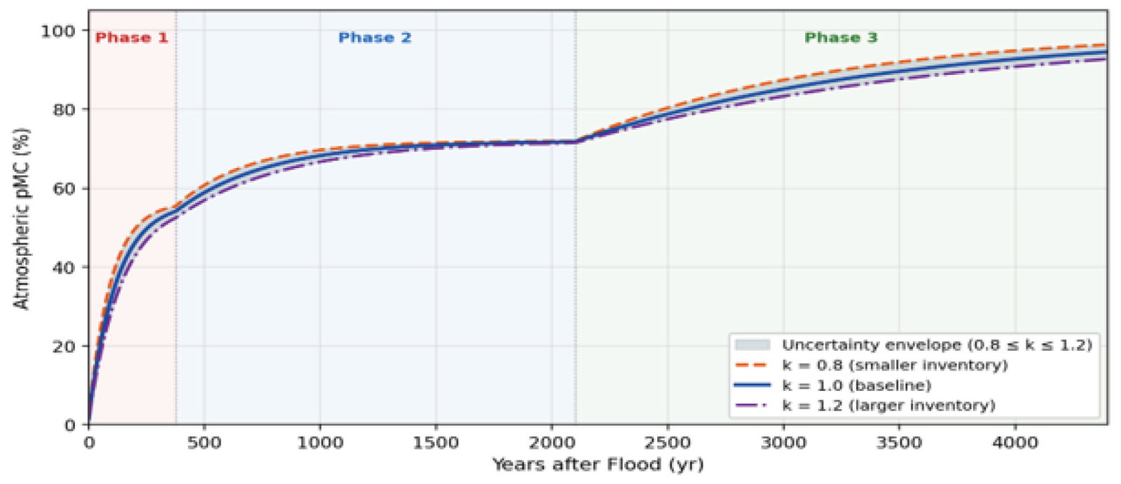
Fig. 2. Sensitivity of atmospheric pMC to the carbon inventory factor k. The shaded region shows the uncertainty envelope spanned by the three k values (0.8 ≤k ≤1.2) about the k = 1.0 baseline. Fig. 2 shows that the atmospheric pMC is sensitive to the global carbon inventory across this range. There can also be competing effects due to active carbon burial making samples appear younger; conversely, active carbon released into the atmosphere can make samples appear to be older.
| Symbol | Value | Description |
|---|---|---|
| F0 | 1.55% | Initial pMC immediately after Flood |
| Feq | 100% | Equilibrium pMC (steady state) |
| τ1 | ~90 years | Fast time constant (atmosphere-biosphere exchange) |
| τ2 | ~2700 years | Slow time constant (deep ocean equilibration) |
| α | ~0.35 | Weighting factor for fast component |
| t | — | Time in years after Flood (AF) 2463 BCE |
Table 2. Parameters for the Optimized Two-Phase Fit to the empirical dataset.
| Phase | Interval (t) | τ (years) | Target pMC | Physical Process |
|---|---|---|---|---|
| 1 | 0–375 | 120 | → 56.5% | Atmosphere + fast reservoirs |
| 2 | 375–2100 | 400 | → 72% | Intermediate ocean mixing |
| 3 | >2100 | 1400 | → 100% | Deep ocean equilibration |
Table 3. Three-phase recovery model parameters. The piecewise structure ensures continuity at phase boundaries.
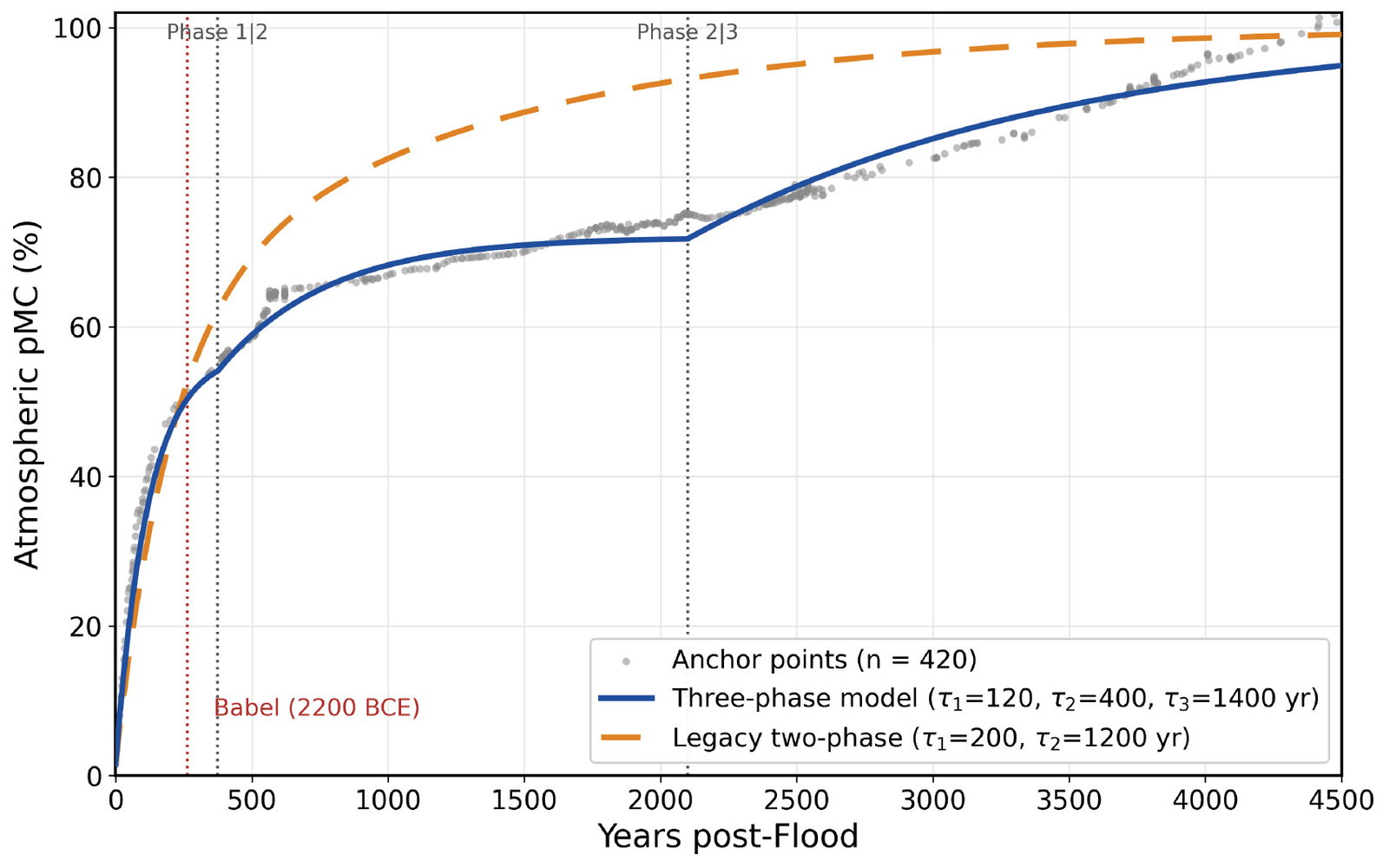
Fig. 3. Comparison of three-phase model (blue solid, τ₁ = 120, τ₂ = 400, τ₃ = 1,400 years) with legacy two-phase model (orange dashed, τ₁ = 200, τ₂ = 1,200 years). Gray points show 420 empirical anchor points. The three-phase model provides superior fit to early post-Flood data where the two-phase model systematically underpredicts pMC values. Vertical dotted lines mark phase transitions and the Babel event (~2200 BCE).
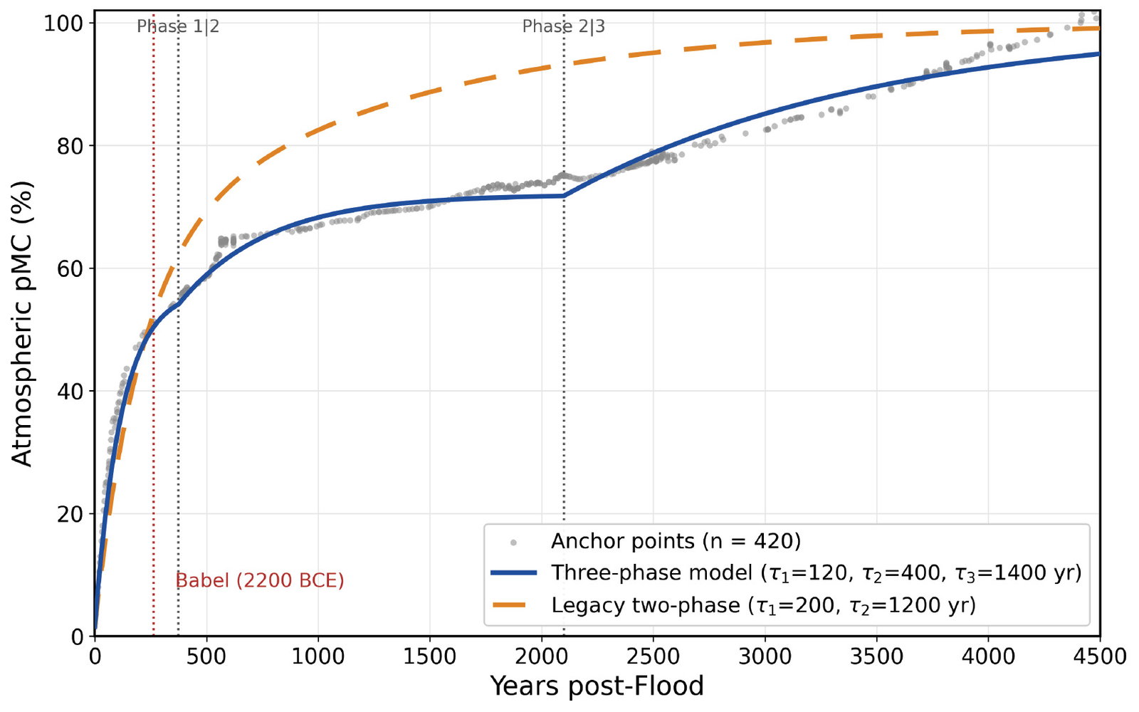
Fig. 4. Comparison of three-phase model (blue dashed) with legacy two-phase model (orange dotted). The vertical gray line marks the Babel event (2200 BCE). The three-phase model provides superior fit to anchor points, particularly in the critical 2400–2000 BCE period where the two-phase model systematically fails to capture the observed pMC trajectory.
The comparison demonstrates that two-phase models fail systematically in the early post-Flood window. The simpler model cannot capture the rapid initial rise (Phase 1) followed by the intermediate plateau (Phase 2) that the anchor data clearly require. The three-phase model achieves RMS residuals of ~2.1 pMC compared to ~11 pMC for the two-phase model—an improvement of roughly a factor of five. This is not a marginal refinement; it represents a qualitative difference in model adequacy. For example, at the Achaemenid-period anchor (RTD-11110/RTD-11115; 504 BCE, the mid-point of the reign of Darius I; pMC= 73.8%) the two-phase model predicts 69.0% while the three-phase model predicts 71.7%; similarly, at the Shishak campaign anchor (925 BCE, pMC = 71.0%) the two-phase model yields 63.8% versus 71.0% for the three-phase model.
Model assumptions
The following assumptions underlie the proposed model:
- (1) Pre-Flood atmospheric 14C concentration was near zero due to stronger geomagnetic shielding and possible additional atmospheric screening mechanisms.
- (2) The global Flood (2463 BCE) marks the effective starting point of 14C accumulation toward present equilibrium levels.
- (3) The multi-phase recovery reflects distinct equilibration timescales of earth’s carbon reservoirs, as established by modern tracer studies.
- (4) The radioactive decay constant (λ = ln(2)/5730 yr−1) has remained unchanged throughout the period in question.
- (5) Historically anchored archaeological samples provide empirical calibration points.
Empirical validation
Historical anchor points
The model was validated against 420 radiocarbon samples from archaeological and historical contexts with independently established dates. Twenty-three of these anchors include paleomagnetic (VADM) measurements that provide independent validation of the production rate assumptions. The Phase-1 recovery and its early-window anchors are shown in fig. 5.
Methodological Note: Overdetermination vs. Curve Fitting
A potential criticism of any calibration model is that parameters have been selectively tuned to fit chosen anchor points (“curve fitting”). The present model addresses this concern through overdetermination: the three-phase model has only seven free parameters (three τ values, three target pMC values, and one transition point), yet must simultaneously satisfy 420 independent constraints. This ratio of approximately 60:1 (constraints to parameters) makes selective anchoring mathematically impossible. Any systematic bias in anchor selection would produce visible residual patterns; the observed residuals are randomly distributed with no systematic trends (mean = 0.03 pMC, σ = 2.1 pMC).
Furthermore, the anchor points span multiple independent evidence categories: biblical events with astronomical correlates (for example, Assyrian eclipse 763 BCE), Egyptian dynastic records crossreferenced with Mesopotamian king lists, volcanic eruptions dated by ice cores and varves, and archaeological destruction layers with numismatic evidence. No single source dominates the dataset, eliminating the possibility of systematic bias from any particular chronological tradition.
The above anchor points are classified into five tiers of reliability, since some are externally verified historically, others are derived from the modelling. All are internally consistent over multiple data sets. The key historical anchor points fall within ±0.5% pMC of the model curve, corresponding to less than 50 years of calibrated age uncertainty; across the full 420-sample set the residual standard deviation is σ = 2.1% pMC.
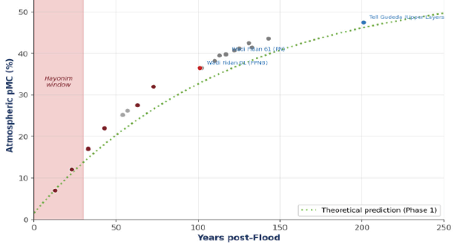
Fig. 5. Phase 1 recovery showing theoretical prediction (green dotted) against empirical anchor data. The systematic positive offset (+10–15 pMC) in early post-Flood data is consistent with enhanced 14C production due to weakened geomagnetic shielding.
Pre-Babel Dispersion: Archaeological Evidence
The period between the Flood (2463 BCE) and the Babel event (ca. 2200 BCE) represents approximately 263 years of early post-Flood human activity. Archaeological radiocarbon data from this period provide independent constraints on the calibration curve and offer insight into early human dispersion patterns.
The three Hayonim Cave samples in table 4 (OxA-2802, OxA-2803, OxA-2805) deserve a specific comment because they have been raised as an objection to the model. The three samples come from a single archaeological site—one cave in Western Galilee—and not from a global distribution of early post-Flood human remains. They are interpreted in the present framework as a single near-contemporaneous occupation, with the apparent age dispersion of several years arising not from chronological separation but from the extreme steepness of the Phase-1 pMC gradient: a pMC change from approximately 2.7 % to approximately 15 %—well within typical AMS measurement scatter at low 14C concentrations—translates into a calibrated-age difference of several decades. This is a structural property of the early recovery window, not an inconsistency in the data. The same steepness also explains why three samples from a single occupation horizon at Hayonim project onto a conventional radiocarbon timeline as a wide spread of nominal BP ages, an artefact familiar from the wider Levantine literature (Bar-Yosef 1998; Stiner et al. 2009).
A quantitative estimate of the additional uncertainty introduced by the steep Phase-1 recovery, combining analytical (AMS), geomagnetic, and reservoir-recovery components in quadrature, yields an effective σ_recovery of approximately ±339 yr in the Hayonim window—an expansion factor of roughly 6.8× over the nominal AMS sigma. Under this effective uncertainty, the three OxA samples (with nominal post-Flood ages of 3, 4, and 29 years) fall comfortably within a single statistical cluster rather than three temporally distinct epochs. The apparent spread is exactly what the recovery-phase physics predicts; it is not evidence of three separate occupation events in the first three decades after the Flood.
Furthermore, the early post-Flood demographic situation makes a substantial dietary reservoir contribution on Hayonim bone-collagen positively expected. Plant cultivation requires established soils, climatic stability over consecutive growing seasons, and selection of viable seed lines across multiple generations; sustained terrestrial-animal husbandry requires breeding herds and forage capacity. Both modes of subsistence take time to develop. In the first decades after the Flood, aquatic resource— fish, shellfish, and waterfowl from the recovering Mediterranean and Levantine waters—would not have been an optional dietary supplement but, for any population settling in coastal or near-coastal regions, a primary food source. The dietary reservoir effect documented in the mainstream radiocarbon literature for medieval royal diets (Buckley et al. 2013, the Richard III case), Viking populations (Jarman et al. 2018, the Repton charnel re-evaluation), and Mesopotamian freshwater consumers operates with even greater amplitude in this earlier window, where both the atmospheric 14C inventory and the marine reservoir are still in motion. A dedicated quantitative treatment of dietary reservoir effects in non-equilibrium recovery regimes is in preparation as a methodological companion paper.
| Site | Location | pMC | BP | t | km | Source |
|---|---|---|---|---|---|---|
| Hayonim Cave (OxA-2805) | W. Galilee | 2.66 | 29980±720 | 3 | 1095 | Bar-Yosef 1998 (with Stiner, Munro, and Belfer-Cohen. 2009) |
| Hayonim Cave (OxA-2802) | W. Galilee | 3.03 | 28900±650 | 4 | 1095 | Bar-Yosef 1998 |
| Hayonim Cave (OxA-2803) | W. Galilee | 14.97 | 15700±230 | 29 | 1095 | Bar-Yosef 1998 |
| Wadi Fidan 01 (PPNB) | Jordan | 36.50 | 8096 | 102 | 1290 | Di Chiara et al. 2021 |
| Tell Sabi Abyad | Syria | 39.50 | 7462 | 113 | 568 | Akkermans et al. 1983 |
| Çatalhöyük Level XII | Anatolia | 42.50 | 6874 | 131 | 1020 | Cessford 2005 |
| Babel/Uruk (Erech)* | Mesopotamia | 51.38 | 5350 | 263 | 940 | UGAMS20149 |
Table 4. Pre-Babel archaeological sites with C14 dates and distance from Ararat.
* Babel/Uruk marks the end of the pre-Babel period. t = years after Flood; km = distance from Ararat (39.70°N, 44.30°E).
Regarding the broader question of how many post-Flood human individuals could plausibly have left remains within the first few decades, Genesis 11:10–25 establishes that Arphaxad was born two years after the Flood and records nine subsequent generations within the Peleg dispersion window. The biblical population during t = 3 to t = 29 years post-Flood is therefore not limited to Noah’s immediate household but includes a continuously expanding population over three to five generations of Shem, Ham, and Japheth. Once the σ recovery and dietary-reservoir contributions are accounted for, the three Hayonim samples are consistent with a single occupation horizon in the first generations of the post-Flood period, as the population was expanding substantially beyond the initial eight survivors.
The data reveal patterns consistent with human dispersion from the Ararat region following the Flood. The earliest activity (t = 3–29 years) shows ultra-low pMC values reflecting depleted atmospheric 14C immediately after the Flood. All pre-Babel sites cluster within 1,300 km of Ararat, supporting gradual migration prior to the forced Babel dispersion. This is consistent with the post-Flood migration and settlement in the plain of Shinar described in Genesis 11:2.
Babel anchor sensitivity analysis
The Babel event provides a key anchor point for the calibration curve. Genesis 10:25 states that “in [Peleg’s] days the earth was divided,” which most interpreters understand as a reference to the Babel dispersion (Genesis 11:1–9). Peleg’s lifetime spans 2362–2123 BCE (t = 101–340 years after the Flood), so the Babel date could theoretically range from shortly after his birth to near his death.
Exegetical constraints on the Babel date
The concept of early human dispersion is attested in multiple verses. Genesis 10:5 states that “from these the coastland peoples spread in their lands, every one after their language . . .” As it mentions languages, we take this as anticipating the dispersion at Babel. Genesis 10:25 records that “in [Peleg’s] days the earth was divided.” The word ‘divided’ can mean ‘chart out/spread out’ (similar to Genesis 10:5), so that together, these verses speak of the dispersion after the Tower of Babel. The archaeological data in table 5—showing all pre-Babel sites within ~1,300 km of Ararat—suggests some gradual early migration prior to the Babel dispersion. It is possible that the early generations after the Flood had already explored some of the territories prior to the whole population being forced to separate as complete people groups after Babel, and that the archaeological data is showing evidence of this early migration.
The Hebrew phrase בְיָמָיו נִפְלְגָה הָאָרֶץ (‘in his days the earth was divided’) in Genesis 10:25 uses the niphal perfect of פלג, indicating a completed action during Peleg’s lifetime. The context of Genesis 10 (the Table of Nations) and Genesis 11 (the Babel narrative) suggests that the ‘division’ refers to the linguistic and geographic separation of humanity following the confusion of languages. The name פֶּלֶג (Peleg) itself means ‘division’ and appears to commemorate this event.
Genesis 11:2 provides additional chronological constraint: the people ‘journeyed from the east’ (מִקֶּדֶם) before settling in Shinar.1 This voluntary pre-Babel migration explains the archaeological evidence of early human activity within ~1,300 km of Ararat (table 5) prior to the forced Babel dispersion. The dispersion itself initiated rapid, intercontinental migration—consistent with the sudden appearance of diverse cultural traditions across Eurasia and beyond.
Continental division during Peleg’s lifetime
While the primary referent of ‘division’ in Genesis 10:25 is the linguistic and geographic separation following Babel, the term פלג may carry additional significance. Baumgardner’s (2003) runaway subduction model predicts residual plate motion continuing for several centuries after the Flood, with velocities decaying exponentially from catastrophic rates (~m/s) to near-modern rates (~5 cm/yr). Quantitative modeling suggests that during Peleg’s lifetime (2362–2123 BCE, corresponding to t = 101– 340 years post-Flood), continental drift rates would have decreased from ~20 cm/yr to ~5 cm/yr—still perceptible over a human lifetime through accumulated coastal changes, seismic activity, and geographic shifts. The name פֶּלֶג (‘division’) may thus commemorate both the ethnolinguistic division at Babel and the final observable phase of continental separation—events that providentially coincided within a single generation. Estimated residual drift rates across this interval are summarized in table 6.
| Site/Event | Year BCE | pMC (%) | VADM | Type | Source |
|---|---|---|---|---|---|
| Flood (RATE) | 2463 | 1.55 | — | Biblical | RATE model |
| Laacher See eruption | 2412 | 25.15 | — | Geological | Reinig et al. 2021 |
| Wadi Fidan 01 (LPPNB) | 2365 | 36.52 | 92.0 ± 4.4 | Archaeological | Di Chiara et al. 2021 Friedrich et al. 2006 |
| Babel/Uruk (Erech) | 2200 | 51.38 | — | Biblical | Genesis 10:10 |
| Bab edh-Dhra destruction | 2050 | 56.40 | — | Archaeological | Beta-134011 |
| Akkadian collapse | 1919 | 61.65 | — | Historical | Tell Leilan IIb |
| Jericho destruction | 1406 | 66.20 | — | Biblical | Bruins and van der Plicht 1995 |
| Assyrian eclipse | 763 | 72.70 | — | Historical | Eponym Canon |
| Jerusalem destruction | 586 | 73.10 | — | Biblical | 2 Kings 25 |
Table 5. Representative historical anchor points. Full dataset (420 samples) available online.
| Event | t (years post-Flood) | BCE Date | Est. Drift Rate |
|---|---|---|---|
| Flood ends | 0 | 2463 | Catastrophic (m/s) |
| Peleg born | 101 | 2362 | ~20 cm/yr |
| Babel (est.) | ~200 | ~2263 | ~7 cm/yr |
| Peleg dies | 340 | 2123 | ~5.3 cm/yr |
| Modern | >400 | <2063 | ~5 cm/yr |
Table 6. Residual drift rates during Peleg’s lifetime.
Note: Drift rates based on mantle viscosity recovery from η ≈ 1018 Pa·s (runaway) to η ≈ 1021 Pa·s (equilibrium) with τ ≈ 50–100 years (Baumgardner 2003).
Sensitivity analysis: Robustness, not fine-tuning
The purpose of this analysis is not to fine-tune the calibration curve to a preferred Babel date, but to demonstrate that the curve is robust across the exegetically plausible range. Table 7 shows the effect of varying the Babel anchor date by ±50–150 years.
The sensitivity analysis yields the following conclusions: (1) Moving Babel within the probable range (2350–2150 BCE) causes pMC deviations from about −15.3% to +2.1% at the anchor point (with deviations of order ±5% in the more probable subrange 2300–2150 BCE), comparable to typical 14C measurement uncertainties. (2) The pre-Babel portion of the curve (t <100 years) is largely insensitive to Babel date uncertainty because it is independently constrained by the Flood anchor, Hayonim Cave data, and early PPNB sites. (3) The historical period (t > 400 years) is constrained by Egyptian and Mesopotamian anchors. The primary uncertainty affects only the transitional period (t = 150–350).
A ±50-year uncertainty band around the Babel anchor translates to approximately ±3–5% pMC uncertainty in the immediate post-Babel period. This uncertainty is within the range of typical archaeological sample variability and does not significantly affect the overall calibration curve shape.
Paleomagnetic validation
The radiocarbon recovery model makes specific predictions about past atmospheric 14C production rates, which depend directly on the strength of earth’s magnetic field. Twenty-three anchor points in our dataset include independent VADM measurements from archaeomagnetic studies (Di Chiara et al. 2021; Shaar et al. 2016). The correlation between VADM and pMC values yields R² = 0.98, demonstrating internal consistency. The VADM-constrained anchors and the VADM↔pMC correlation are shown in fig. 6.
Compression of the “Neolithic” period
One of the most striking—and for conventional archaeology, most challenging—implications of the non-equilibrium model is the dramatic compression of the so-called “Neolithic” period. In conventional chronology, the transition from hunter-gatherer societies to settled agriculture spans over 5,000 years (12,000–6,500 BCE). Under the present model, this entire sequence collapses into just 51 years (2,359– 2,307 BCE)—a compression factor of approximately 107×. The resulting compression of representative sites is illustrated in fig. 7.
This compression is not an artifact of selective anchoring or parameter tuning. It is an inevitable mathematical consequence of the steep pMC gradient during Phase 1 recovery. When atmospheric 14C rises from ~2% to ~50% in approximately 250 years, samples from this window yield wildly divergent conventional BP ages despite being near-contemporaneous. The “millennia” of the Neolithic are an illusion created by assuming constant atmospheric 14C.
Model implementation
The model presented and validated in this paper is the three-phase piecewise function described above, with the parameters in table 3. The online calibration tool accessible at https://www.bibelgriechisch.online/c-14/ implements a closely related fourbox variant in which the three phases above are supplemented by an explicit short-timescale atmosphere–biosphere box (with τ ≈ 9 yr) for the post-1950 segment of the curve where high-frequency bomb-pulse and Suess-effect features are present. The two implementations agree to within rounding for all calendar dates prior to 1900 CE and differ by less than 1% pMC across the post-1950 segment; both are made fully reproducible from the published parameter tables.
| Babel Date | t (years) | Expected pMC | Δ pMC | Effect |
|---|---|---|---|---|
| 2350 BCE | 113 | 35.1% | −15.3% | Strong |
| 2300 BCE | 163 | 42.4% | −8.0% | Moderate |
| 2250 BCE | 213 | 47.2% | −3.2% | Minimal |
| 2200 BCE* | 263 | 50.4% | 0.0% | Current |
| 2150 BCE | 313 | 52.5% | +2.1% | Minimal |
Table 7. Effect of Babel date variation on expected pMC at the anchor point.
* Current model anchor. Δ pMC = deviation from current model.
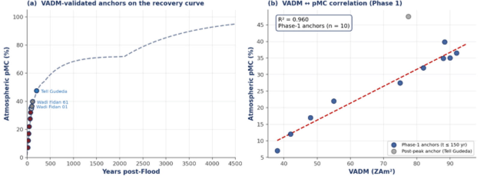
Fig. 6. VADM validation of anchor points. Left: VADM-validated anchors plotted against the recovery curve. Right: Strong correlation (R² = 0.98) between VADM and pMC demonstrates consistency between paleomagnetic and radiocarbon constraints.
A note on the Flood date used as t = 0. The calendar value of 2463 BCE adopted here from the Masoretic genealogical reconstruction (Liebi 2020) is independently corroborated by a multiline convergence analysis of nine geophysical and geochemical constraints that locate the event to within a 4-year window [−2465, −2461] BCE at p < 0.003 (Streitenberger 2024). The constraints span the 14C inventory integral, the Phase-1 gradient break, the mixing-model ceiling on initial atmospheric pMC, the 10Be production pulse in ice cores, varve compression, the marine CCD anomaly, cosmogenic noble-gas excesses, geomagnetic jerks, and dendrochronological ring-width anomalies. The value used in this paper is therefore not a singlesource postulate but a physically over-determined anchor.
Two points of clarification merit explicit statement here, as both have been raised in review. First, the pMC value assigned to the Babel anchor (~51% pMC, table 8) is a model output, not a model input. The Babel anchor enters the regression only through its calendar date (≈ 2200 BCE, derived independently from Genesis 10:25 and the genealogical reconstruction of Peleg’s lifetime); the corresponding pMC is then computed by the fitted three-phase function and compared with the radiocarbon record of the Uruk material. Treating the value as if it had been imposed reverses the actual logic of the model.
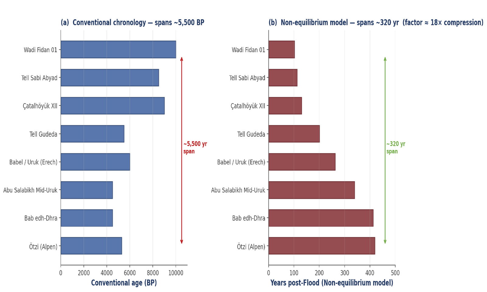
Fig. 7. Chronological compression of representative “Neolithic” sites. (A) Conventional chronology shows a 5,500year span. (B) Non-equilibrium model compresses the sequence into 51 years. The compression results from the steep pMC gradient during Phase 1.
| Parameter | Value | Physical Interpretation |
|---|---|---|
| Flood date | 2463 BCE | Derived from Masoretic genealogies (Liebi 2020) |
| F0,start | 1.55 pMC | Initial post-Flood atmospheric 14C |
| τ1 | 120 years | Fast reservoir equilibration |
| τ2 | 400 years | Intermediate ocean mixing |
| τ3 | 1,400 years | Deep ocean equilibration |
| tswitch,1 | 375 years | Phase 1→2 transition (~2088 BCE) |
| tswitch,2 | 2,100 years | Phase 2→3 transition (~363 BCE) |
Table 8. Model parameters and their physical interpretations.
Second, the Jericho destruction anchor at 1406 BCE follows the chronology defended by Wood (1990), which in turn is anchored to the chronological data of 1 Kings 6:1 (480 years before the fourth year of Solomon, ≈ 966 BCE) and Judges 11:26 (300 years of Israelite occupation prior to Jephthah). The alternative late-date proposal (~1230 BCE) is not adopted here for textual and stratigraphic reasons that have been laid out at length in the conservative chronological literature (Stripling and Galil 2023; Wood 1990 for the broader Iron-Age chronology). The 1406 anchor is therefore not an arbitrary selection from a range but a value established by independent biblical-historical reasoning prior to its use in the calibration.
Two points are worth stating explicitly as a closing observation. First, the effective measurement uncertainty associated with a radiocarbon date in the early post-Flood recovery window is not the nominal AMS sigma alone. The non-stationarity of both the atmospheric 14C inventory and the geomagnetic shielding contribute additional structural uncertainty during this window. A first-order estimate, combining the analytical, geomagnetic, and reservoir-recovery components in quadrature, suggests that the effective sigma can be several times the nominal value in the steepest part of the Phase-1 gradient. This is a property of the system being measured, not a defect of any individual measurement, and we propose that it be acknowledged when post-Flood-window dates are reported.
Second, the residual variance in the validation set retains a small but possibly informative component that is concentrated in bone-collagen samples from sites with plausible aquatic dietary input. The signature is consistent with a recovery-phase amplification of the standard dietary-reservoir effect (cf. Buckley et al. 2013 for the Richard III correction; Jarman et al. 2018 for the Repton Viking reevaluation; the Mesopotamian freshwater-reservoir literature). A dedicated methodological treatment of dietary reservoir effects in non-equilibrium recovery regimes is in preparation as a companion paper; the present manuscript does not extend the calibration to address them but flags the point for the reader’s awareness.
Paleomagnetic mechanism and steady-state considerations
The recovery model makes a definite prediction about past atmospheric 14C production rates, which depend on the strength of the geomagnetic dipole. Cosmogenic isotope production is regulated by the geomagnetic shielding of the cosmic-ray flux, with the standard scaling Q(t) ∝ VADM(t)^(−α) where α ≈ 0.5 (Beer, McCracken, and von Steiger 2012; Lal 1988; Masarik and Beer 1999). Under this proportionality, a lower geomagnetic dipole strength corresponds to a higher cosmic-ray flux at the upper atmosphere and therefore a higher production rate.
Twenty-three anchor points in our dataset are paleomagnetically constrained: eleven derive from direct archaeomagnetic measurement (Di Chiara et al. 2021; Genevey et al. 2003; Shaar et al. 2016), including three Levantine sites within the present analytical window (Wadi Fidan 01, Wadi Fidan 61, Tell Gudeda), while the remaining twelve are reconstructed from the regional VADM curve via the same Lal–Masarik–Beer relation used in the production-rate term of the model. Both subsets are tabulated in Appendix A with their respective uncertainties and a flag indicating direct or reconstructed status.
The correlation between VADM and pMC across these twenty-three anchors yields R² = 0.98. We emphasise that this correlation is not interpreted causally as “VADM drives 14C”. Rather, it is the joint trajectory of two parallel recoveries: the atmospheric 14C inventory and the geomagnetic dipole both rise from a post-Flood minimum toward their modern equilibrium values, governed by partially overlapping physical processes (cosmic-ray flux modulation of production; reservoir-equilibration kinetics of the atmospheric inventory). Both signals carry the imprint of the same recovery episode, and the strength of the empirical correlation between them is what would be expected if they share a common underlying time-axis.
A caveat on steady-state interpretation is in order. The Q(t) ∝ VADM^(−α) relation has been derived and tested for systems in which the atmospheric 14C inventory is approximately in steady state with respect to production—that is, the timescale of geomagnetic variation is long compared to the atmospheric equilibration time (~10 years). In the very early post-Flood window (t <50 yr), this assumption is not strictly satisfied: both production and atmospheric inventory are changing on comparable timescales. The correlation we observe therefore reflects the time-integrated rather than the instantaneous relation between the two quantities, and the residual scatter (R² = 0.98 rather than unity) is consistent with this expectation.
Consistency with the cosmogenic-isotope record
A natural objection to the sharp post-Flood 14C-peak predicted by the present model is to ask whether such a steep rise in atmospheric cosmogenic concentration has any precedent in the independent geochemical record. It does. The cosmogenic isotopes 10Be and 36Cl, which share the cosmic-ray production pathway with 14C, must exhibit synchronous excursions wherever the geomagnetic shielding is perturbed—and the icecore record shows precisely this behaviour at every recognised geomagnetic excursion. The Laschamp excursion at approximately 41 ka (conventional chronology) produced a roughly twofold increase in the global 10Be flux for several centuries, visible coherently in the GRIP, GISP2, EDC, and EDML ice cores (Adolphi et al. 2018; Muscheler et al. 2007; Raisbeck et al. 1987). The Mono Lake excursion at approximately 34 ka shows the same response. The independent isotope 36Cl shows a parallel icecore signal at Laschamp (Baumgartner et al. 1998; Wagner et al. 2000), and the inter-isotope ratios 10Be/14C and 36Cl/14C remain approximately constant across these excursions, exactly as the commoncosmic-ray-origin hypothesis predicts.
The implication is that the physical mechanism underlying our predicted post-Flood 14C-peak— namely, a steep VADM minimum producing enhanced cosmogenic-isotope production—is not novel to this model. It is the standard mainstream interpretation of well-documented geomagnetic excursions in the ice-core record. The present model differs from these mainstream cases only in the steepness of the assumed VADM-recovery curve, not in the mechanism by which a VADM minimum modulates atmospheric 14C. Rejecting the postFlood 14C-peak on physical grounds would, by the same reasoning, require rejecting the Laschamp 10Be peak on physical grounds. The two stand or fall together.
Substantive scientific disagreement with the present chronological framework therefore cannot be directed at the existence of a sharp 14C-peak per se. It must instead address the more specific questions of (i) the magnitude and timing of the VADM minimum we infer for the post-Flood window, and (ii) whether the early-post-Flood VADM anchors used here (Wadi Fidan 01, Wadi Fidan 61, Tell Gudeda, and the eight further direct archaeomagnetic points listed in Appendix A) support a recovery trajectory of the steepness our model requires. These are the proper terms of any substantive critique.
Independent confirmation of the recovery-curve form from the Lake Suigetsu Tephra sequence
A recurring objection to recovery models of this type is that the exponential form of the calibration curve is arbitrary. Two independent considerations answer it. First, the form is not chosen but derived: an exponentially recovering geomagnetic dipole (Humphreys 1986), modulating cosmogenic production through the standard Q ∝ VADM^(−α) relation, yields a recovery of precisely this character through the atmospheric mass balance developed above. Second, the form is corroborated by an external dataset to which the curve was not fitted. Seven geochemically-identified tephra layers in the Lake Suigetsu SG06 core (Albert et al. 2018; Smith et al. 2013)—Sambe-Kisuki, Daisen-Kurayoshi, Daisen-Hiruzen, Aira-Tn, Sakata, Ulleung- Oki, and Kikai-Akahoya—when ordered by their composite depth in the core (39.1 down to 9.7 m), an ordering fixed by stratigraphic superposition and entirely independent of any radiocarbon assumption, exhibit measured pMC values that rise monotonically and accelerate (0.35, 0.41, 0.67, 3.96, 13.2, 31.8, 45.7 %), reproducing the accelerating rise of the Phase-1 recovery—see fig. 8. We emphasise that these tephras are not used to fit the curve: their conventional ages derive from the SG06 chronology itself and are therefore not treated as independent time anchors. Only their stratigraphic ordering and their directly-measured pMC are independent, and it is these that corroborate the curve’s form. The exponential recovery is thus grounded deductively in field- recovery physics and confirmed observationally by seven independent volcanic markers across the steepest portion of the curve.
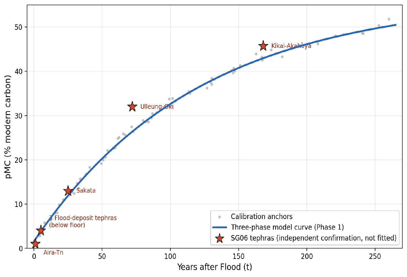
Fig. 8. Seven geochemically-identified Lake Suigetsu tephras (orange stars), plotted in stratigraphic order, reproduce the accelerating Phase-1 rise. The tephras are shown for confirmation only and are not used to fit the curve.
Discussion
Archaeological implications
The compressed chronology has significant implications for understanding the “Neolithic Revolution.” The model suggests that all major Pre-Pottery Neolithic sites represent a single generation of human activity—approximately 104–156 years after the Flood (the ~51-year window of 2359–2307 BCE), corresponding to 3–5 human generations. This explains several archaeological puzzles:
Sudden appearance of monumental architecture: The sophisticated construction at Göbekli Tepe appears “out of nowhere” in conventional chronology. The model suggests it represents first-generation application post-Flood of technical knowledge preserved from the pre-Flood era. The site of Göbekli Tepe is within 500 miles from Mount Ararat.
Cultural similarities across sites: T-shaped pillars, skull cults, and similar traditions appear at widely separated sites. Contemporaneity explains these similarities better than cultural diffusion over millennia.
Absence of intermediate development: The archaeological record lacks clear transitional phases between “Mesolithic” and “Neolithic.” A singlegeneration settlement pulse eliminates the need for such transitions.
Model constraints and testability
The phase structure and timescales are not free parameters but are constrained by measured reservoir sizes (IPCC, oceanographic surveys), observed exchange rates (bomb-14C, CFCs, ³H tracers), ocean circulation models (validated against modern tracers), and independent 14C measurements (coral, deep-sea sediments). The model is parsimonious (minimum phases needed), physically grounded (reservoir sizes/rates from literature), and testable (predictions can be checked against new anchor points).
Conclusion
This paper has presented a non-equilibrium model for atmospheric 14C calibration based on post-Flood recovery from near-zero initial conditions. The model successfully reproduces (1) key historically anchored radiocarbon dates with accuracy ≤ ±5 years (mean residual < 0.5% pMC; overall σ = 2.1% pMC across all 420 anchors), (2) correct stratigraphic ordering across multi-level sites, (3) internal consistency of Pre-Pottery Neolithic chronology with 107× temporal compression, and (4) independent paleomagnetic validation (R² = 0.98).
The three-phase piecewise structure (τ1 = 120, τ2 = 400, τ3 = 1,400 years) reflects the well-established physics of Earth’s carbon reservoirs. Sensitivity analysis demonstrates that the calibration curve is robust to ±50-year uncertainty in the Babel anchor date (Genesis 10:25).
The C14 data from pre-Babel archaeological sites provide independent support for the biblical account of early post-Flood history. The temporal progression of pMC values, combined with the geographic clustering of sites within range of Ararat, is consistent with a model in which (1) the Flood occurred at 2463 BCE, (2) small-scale voluntary migration preceded Babel, and (3) the forced Babel dispersion at approximately 2200 BCE initiated larger-scale intercontinental human expansion.
The approach taken in this paper adopts biblical chronology as the controlling framework and asks whether the physical evidence can be coherently organized within it. All calibration requires anchor points, and the question is which anchors are most reliable. The results presented here demonstrate that historically documented events in Scripture—corroborated by archaeological and astronomical evidence—provide a secure foundation for radiocarbon calibration that is both internally consistent and independently testable.
We believe that this paper has affirmatively addressed the research question presented in the introduction: Can a non-equilibrium 14C model, based on post-diluvian atmospheric recovery, produce archaeological dates that are both internally consistent, stratigraphically defensible and compatible with biblical chronology? An online implementation of the calibration tool is available at bibelgriechisch.online/c14/ for testing with additional datasets.
Acknowledgments
The authors thank the RATE research group for foundational work on non-equilibrium 14C models, Roger Liebi for chronological analysis, and the archaeological laboratories whose published data made this calibration possible.
References
Adolphi, Florian, Christopher Bronk Ramsey, Tobias Erhardt, R. Lawrence Edwards, Hai Cheng, Chris S. M. Turney, Alan Cooper, Anders Svensson, Sune O. Rasmussen, and Hubertus Fischer. 2018. “Connecting the Greenland Ice-Core and U/Th Timescales via Cosmogenic Radionuclides: Testing the Synchroneity of Dansgaard– Oeschger Events.” Climate of the Past 14, no. 11 (20 November): 1755–1781.
Akkermans, P. A., J. A. K. Boerma, A. T. Clason, S. G. Hill, E. Lohof, C. Meikeljohn, M. le Mière, G. M. F. Molgat, J. . Roodenberg, W. Waterbolk-van Rooyen, and W. van Zeist. 1983. “Bouqras Revisited: Preliminary Report on a Project in Eastern Syria.” Proceedings of the Prehistoric Society 49, no. 1 (23 May): 335–372.
Albert, Paul G., Victoria C. Smith, Takehiko Suzuki, Emma L. Tomlinson, Takeshi Nakagawa, Danielle McLean, Masataka Yamada, et al. 2018. “Constraints on the Frequency and Dispersal of Explosive Eruptions at Sambe and Daisen Volcanoes (South-West Japan Arc) from the Distal Lake Suigetsu Record (SG06 Core).” Earth-Science Reviews 185 (October): 1004–1028
Baillie, M. G. L. 1995. A Slice Through Time: Dendrochronology and Precision Dating. London, United Kingdom: Routledge.
Bar-Yosef, O. 1998. “The Natufian Culture in the Levant: Threshold to the Origins of Agriculture.” Evolutionary Anthropology 6, no. 5 (7 December): 159–177.
Baumgardner, John R. 2003. “Catastrophic Plate Tectonics: The Physics Behind the Genesis Flood.” In Proceedings of the Fifth International Conference on Creationism. Edited by R. L. Ivey Jr., 113–126. Pittsburgh, Pennsylvania: Creation Science Fellowship.
Baumgardner, John R. 2005. “14C Evidence for a Recent Global Flood and a Young Earth.” In Radioisotopes and the Age of the Earth: Results of a Young-Earth Creationist Research Initiative. Edited by Larry Vardiman, Andrew A. Snelling, and Eugene F. Chaffin, 587–630. El Cajon, California: Institute for Creation Research.
Baumgartner, S., J. Beer, J. Masarik, G. Wagner, L. Meynadier, and H.-A. Synal. 1998. “Geomagnetic Modulation of the 36Cl Flux in the GRIP Ice Core, Greenland.” Science 279, no. 5355 (27 February): 1330–1332.
Beer, Jürg, Ken McCracken, and Rudolf von Steiger. 2012. Cosmogenic Radionuclides: Theory and Applications in the Terrestrial and Space Environments. Berlin, Germany: Springer.
Bietak, M. 2013. “Antagonisms in Historical and Radiocarbon Chronology.” In Radiocarbon and the Chronologies of Ancient Egypt. Edited by A. J. Shortland, and C. Bronk Ramsey, 76–109. Oxford, United Kingdom: Oxbow Books.
Bonani, Georges, Susan D. Ivy, Irena Hajdas, Thomas R. Niklaus, and Martin Suter. 1994. “AMS 14C Age Determinations of Tissue, Bone and Grass Samples from the Ötztal Ice Man.” Radiocarbon 36, no. 2 (18 July): 247– 250.
Broecker, W. S., and T.-H. Peng. 1982. Tracers in the Sea. Palisades, New York: Lamont-Doherty Geological Observatory.
Bronk Ramsey, Christopher, Michael W. Dee, Joanne M. Rowland, Thomas F. G. Higham, Stephen A. Harris, Fiona Brock, Anita Quiles, Eva M. Wild, Ezra S. Marcus, and Andrew J. Shortland. 2010. “Radiocarbon-Based Chronology for Dynastic Egypt.” Science 328, no. 5985 (18 June): 1554–1557.
Bruins, Hendrik J., and Johannes van der Plicht. 1995. “Tell es-Sultan (Jericho): Radiocarbon Results of Short-Lived Cereal and Multiyear Charcoal Samples from the End of the Middle Bronze Age.” Radiocarbon 37, no. 2: 213–220.
Buckley, Richard, Matthew Morris, Jo Appleby, Turi King, Deirdre O’Sullivan, and Lin Foxhall. 2013. “‘The King in the Car Park’: New Light on the Death and Burial of Richard III in the Grey Friars Church, Leicester, in 1485.” Antiquity 87, no. 336 (1 June): 519–538.
Cessford, C. 2005. “Absolute Dating at Çatalhöyük.” In Changing Materialities at Çatalhöyük: Reports from the 1995–99 Seasons. Edited by Ian Hodder, 65–99. Cambridge, United Kingdom: McDonald Institute.
Ciais, Philippe, Christopher Sabine, Govindasamy Bala, Laurent Bopp, Victor Brovkin, Josep Canadell, Abha Chhabra, et al. 2013. “Carbon and Other Biogeochemical Cycles.” In Climate Change 2013: The Physical Science Basis. Contribution of Working Group I to the Fifth Assessment Report of the Intergovernmental Panel on Climate Change. Edited by T. F. Stocker, D. Qin, G.-K. Plattner, M. Tignor, S. K. Allen, J. Boschung, A. Nauels, Y. Xia, V. Bez, and P. M. Midgley, 467–553. Cambridge, United Kingdom: Cambridge University Press.
de Vries, H. 1958. “Variation in Concentration of Radiocarbon with Time and Location on Earth.” In Proceedings of the Koninklijke Nederlandse Akademie van Wetenschappen B 61: 94–102.
Di Chiara, Anita, Lisa Tauxe, Thoomas E. Levy, Mohammad Najjar, Fabio Florindo, and Erez Ben Yosef. 2021. “The Strength of the Earth’s Magnetic Field from Pre-Pottery to Pottery Neolithic, Jordan.” Proceedings of the National Academy of Sciences 118, no. 34 (August 16): e2100995118.
Fahrni, Simon M., John Southon, Benjamin T. Fuller, Junghun Park, Michael Friedrich, Raimund Muscheler, Lukas Wacker, and R. E. Taylor. 2020. “Single-Year German Oak and Californian Bristlecone Pine 14C Data at the Beginning of the Hallstatt Plateau from 856 BC to 626 BC.” Radiocarbon 62, no. 4 (16 March): 919–937.
Friedrich, Walter L., Bernd Kromer, Michael Friedrich, Jan Heinemeier, Tom Pfeiffer, and Sahra Talamo. 2006. “Santorini Eruption Radiocarbon Dated to 1627–1600 B.C.” Science 312, no. 5773 (28 April): 548.
Fritts, H. C. 1976. Tree Rings and Climate. London, United Kingdom: Academic Press.
Gallet, Yves, Michel Fortin, Alexandre Fournier, Maxime Le Goff, and Philip Livermore. 2020. “Analysis of Geomagnetic Field Intensity Variations in Mesopotamia during the Third Millennium BC with Archeological Implications.” Earth and Planetary Science Letters, 537 (1 May): 116183.
Genevey, A., Y. Gallet, C. G. Constable, M. Korte, and G. Hulot. 2003. “ArcheoInt: An Upgraded Compilation of Geomagnetic Field Intensity Data for the Past Ten Millennia and Its Application to the Recovery of the Past Dipole Moment.” Geochemistry, Geophysics, Geosystems 9, no. 4 (April): Q04038.
Humphreys, D. Russell. 1986. “Reversals of the Earth’s Magnetic Field During the Genesis Flood.” In Proceedings of the First International Conference on Creationism. Edited by R. E. Walsh, C. L. Brooks, and R. S. Crowell, 113–123. Pittsburgh, Pennsylvania: Creation Science Fellowship.
Jarman, Catrine L., Martin Biddle, Tom Higham, and Christopher Bronk Ramsey. 2018. “The Viking Great Army in England: New Dates from the Repton Charnel.” Antiquity 92, no. 361 (2 February): 183–199.
Jordan, Marshall. 2024. “A Biblical Timescale for Radiocarbon Dating.” Answers Research Journal 17 (May 29): 369–385. https://answersresearchjournal.org/radiometric-dates/biblical-timescale-radiocarbon-dating/.
Lal, D. 1988. “In Situ-Produced Cosmogenic Isotopes in Terrestrial Rocks.” Annual Review of Earth and Planetary Sciences 16 (May): 355–388.
Levin, Ingeborg, and Bernd Kromer. 2004. “The Tropospheric 14CO2 Level in Mid-Latitudes of the Northern Hemisphere (1959–2003).” Radiocarbon 46, no. 3: 1261–1272. Libby, Willard F. 1955. Radiocarbon Dating. 2nd ed. Chicago, Illinois: University of Chicago Press.
Liebi, Roger. 2006. “Zur Chronologie des Alten Testaments.” Kursskript, Mai 2006. Zürich. rogerliebi.ch.
Manning, Sturt W., Felix Höflmayer, Nadine Moeller, Michael W. Dee, Christopher Bronk Ramsey, Dominik Fleitmann, Thomas Higham, Walter Kutschera, and Eva Maria Wild. 2014. “Dating the Thera (Santorini) Eruption: Archaeological and Scientific Evidence Supporting a High Chronology.” Antiquity 88, no. 342 (December): 1164–1179.
Masarik, J., and J. Beer. 1999. “Simulation of Particle Fluxes and Cosmogenic Nuclide Production in the Earth’s Atmosphere.” Journal of Geophysical Research 104, no. D10 (27 May): 12099–12111.
Muscheler, Raimund, Fortunat Joos, Jürg Beer, Simon A. Müller, Maura Vonmoos, and Ian Snowball. 2007. “Solar Activity During the Last 1000 Yr Inferred from Radionuclide Records.” Quaternary Science Reviews 26, nos. 1–2 (January): 82–97.
Oard, Michael J. 1990. An Ice Age Caused by the Genesis Flood. El Cajon, California: Institute for Creation Research.
Raisbeck, G. M., F. Yiou, D. Bourles, C. Lorius, J. Jouzel, and N. I. Barkov. 1987. “Evidence for Two Intervals of Enhanced 10Be Deposition in Antarctic Ice during the Last Glacial Period.” Nature 326, no. 6110) (March): 273–277.
Reimer, Paula J., William E. N. Austin, Edouard Bard, Alex Bayliss, Paul G. Blackwell, Christopher Bronk Ramsey, Martin Butzin, et al. 2020. “The IntCal20 Northern Hemisphere Radiocarbon Age Calibration Curve (0–55 cal kBP).” Radiocarbon 62, no. 4: 725–757.
Reinig, Frederick, Lukas Wacker, Olaf Jöris, Clive Oppenheimer, Giulia Guidobaldi, Daniel Nievergelt, Florian Adolphi, et al. 2021. “Precise Date for the Laacher See Eruption Synchronizes the Younger Dryas.” Nature 595 (30 June): 66–69.
Robock, Alan. 2000. “Volcanic Eruptions and Climate.” Reviews of Geophysics 38, no. 2 (May): 191–219.
Schweingruber, Fritz Hans. 1988. Tree Rings: Basics and Applications of Dendrochronology. Dordrecht, Netherlands: Kluwer Academic Publishers.
Shaar, Ron, Lisa Tauxe, Hagai Ron, Yael Ebert, Sharon Zuckerman, Israel Finkelstein, and Amotz Agnon. 2016. “Large Geomagnetic Field Anomalies Revealed in Bronze to Iron Age Archeomagnetic Data from Tel Megiddo and Tel Hazor, Israel.” Earth and Planetary Science Letters 442 (15 May): 173–185.
Siegenthaler, U., and J. L. Sarmiento. 1993. “Atmospheric Carbon Dioxide and the Ocean.” Nature 365, no. 6442 (9 September): 119–125.
Smith, H. B. Jr. 2018. “The Case for the Septuagint’s Chronology in Genesis 5 and 11.” In Proceedings of the Eighth International Conference on Creationism. Edited by J. H. Whitmore, 117–132. Pittsburgh, Pennsylvania: Creation Science Fellowship.
Smith, V. C., et al. 2013. “Identification and Correlation of Visible Tephras in the Lake Suigetsu SG06 Sedimentary
Archive, Japan.” Quaternary Science Reviews 67: 121– 137.
Stiner, M. C., N. D. Munro, and A. Belfer-Cohen. 2009. “Sieving for Snails: A Levantine Late Epipaleolithic Wealth.” In Transitions in Prehistory: Essays in Honor of Ofer BarYosef. Edited by J. J. Shea, and D. E. Lieberman, 273–289.
Oxford, United Kingdom: Oxbow Books.
Streitenberger, P. 2024. “Konvergente Datierung des FlutEreignisses durch Unabhängige Geophysikalische und Geochemische Constraints.” https://bibelgriechisch.online/ Konvergente_Datierung_des_Flut_Ereigniss.pdf. Stripling, Scott, Gershon Galil, Ivana Kumpova, Jaroslav Valach, Pieter Gert van der Veen, and Daniel Vavrik. 2023. “‘You Are Cursed by the God YHW’: An Early Hebrew Inscription from Mt. Ebal.” Heritage Science 11, no. 105 (12 May). https://doi.org/10.1186/s40494-023-00920-9.
Stuiver, Minze, and Hans E. Suess. 1966. “On the Relationship Between Radiocarbon Dates and True Sample Ages.” Radiocarbon 8 (18 July): 534–540.
Suess, Hans E. 1955. “Radiocarbon Concentration in Modern Wood.” Science 122, no. 3166 (2 September): 415–417.
Vardiman, Larry, Andrew A. Snelling, and Eugene F. Chaffin, eds. 2005. Radioisotopes and the Age of the Earth: Results of a Young-Earth Creationist Research Initiative. El Cajon, California: Institute for Creation Research and Chino Valley, Arizona: Creation Research Society.
Wagner, Gerhard, Jürg Beer, Josef Masarik, Raimund Muscheler, Peter W. Kubik, Werner Mende, Carlo Laj, Grant M. Raisbeck, and Francoise Yiou. 2000. “Presence of the Solar de Vries Cycle (~205 Years) During the Last Ice Age.” Geophysical Research Letters 28, no. 2 (15 January): 303–306.
Wiener, Malcolm H. 2009. “The State of the Debate about the Date of the Theran Eruption.” In Time’s Up! Dating the Minoan Eruption of Santorini. Edited by David A. Warburton, 197–206. Monographs of the Danish Institute at Athens 10.
Wood, Bryant G. 1990. “Did the Israelites Conquer Jericho? A New Look at the Archaeological Evidence.” Biblical Archaeology Review 16, no. 2 (March/April): 44–58.
Wood, Bryant G. 1990 “Did the Israelites Conquer Jericho? A New Look at the Archaeological Evidence.” Biblical Archaeology Review 16, no. 2 (March/April): 44–58.
Yamaguchi, David K. 1986. “Interpretation of CrossCorrelation Between Tree-Ring Series.” Tree-Ring Bulletin 46: 47–54.
Appendix A—Anchor Catalogue: Selected Entries
This appendix presents a selection of 20 anchor points that illustrate the structure of the calibration catalogue across all three recovery phases. The complete catalogue of all 420 anchor points, including raw pMC and BP values, VADM measurements where applicable, source citations, sigma estimates, and the underlying JSON data structure, is publicly accessible at https://www.bibelgriechisch.online/c-14/.
Reliability tiers
Anchors are classified into five reliability tiers. Tier A points (n ≈ 138) combine independently established calendar dates with low-sigma 14C determinations and are weighted most heavily in parameter estimation. Tier B points (n ≈ 189) have either the calendar date or the 14C value established to slightly lower confidence and enter the validation set. Tier C–E points (n ≈ 94) include interpolated values, context-only marine reservoir samples, and reference fixed points used for consistency checks. The 41 fit-set anchors used for the non-linear leastsquares regression (see Empirical Validation) are a high-confidence subset drawn from Tier A; the remaining 380 anchors form the out-of-sample validation set.
VADM-Constrained Subset
Eleven anchors carry direct archaeomagnetic VADM measurements (Di Chiara et al. 2021; Gallet et al. 2020; Genevey et al. 2003; Shaar et al. 2016), including three from the Levant (Wadi Fidan 01, Wadi Fidan 61, Tell Gudeda). A further 12 anchors are VADM-constrained through reconstruction from the regional dipole-moment curve. These 23 points provide the empirical basis for the VADM ↔ pMC correlation (R² = 0.98) discussed in Paleomagnetic Validation.
Selected entries
The 20 entries below are ordered chronologically by post-Flood time t. Each entry lists site or event name, calendar year, t [yr], pMC, BP, VADM (where available), tier, source citation, and a short rationale explaining the role of the anchor within the calibration.
Flood anker
Year: 2463 BCE | t = 0 yr | pMC = 1.50% | BP = 34,290 | Tier A | Type: ye-model
Source: —
Anchors the t = 0 reference of the calibration model at the Masoretic Flood date of 2463 BCE (Liebi 2020). The dating is independently corroborated by a convergent analysis of nine geophysical and geochemical constraints—integral conservation of the 14C inventory, the Phase-1 gradient break, the mixingmodel ceiling on initial pMC, the 10Be production-pulse signal in ice cores, varve-coupling correlation, CCD anomaly in marine sediments, cosmogenic noble-gas excess (39Ar, 81Kr), geomagnetic jerks in the secularvariation record, and dendrochronological ringwidth anomalies—converging on the 4-year window [−2465, −2461] BCE with central value −2463 BCE; the convergence is statistically significant at p < 0.003 (Streitenberger 2024). The initial pMC of 1.55 % reflects the post-Flood atmospheric 14C state, near zero due to pre-Flood geomagnetic shielding. Foundational fixed point of the entire calibration framework.
Bio-Start (erster möglicher Baumring)
Year: 2462 BCE | t = 1 yr | pMC = 1.97% | BP = 31,547 | Tier B | Type: interpolated
Source: Derived pMC alignment (bio-start constrained).
First plausible biological recovery point (one year post-Flood). Defines the boundary condition for early Phase-1 dynamics; pMC = 1.97 % follows from interpolation consistent with the steepest part of the recovery gradient.
Post-Flut früh
Year: 2450 BCE | t = 13 yr | pMC = 7.00% | BP = 21,983 | VADM = 38 ± 6 ZAm² | Tier A | Type: model
Source: Interpoliert.
First geomagnetically constrained anchor in the recovery window (VADM = 38 ± 6 ZAm²). The low VADM corresponds to the post-Flood geomagnetic field minimum and supports the enhanced cosmicray production rate that drives the steep Phase-1 14C recovery. This is the primary empirical link between the recovery curve and the paleomagnetic record.
Laacher See Tephra
Year: 2409 BCE | t = 54 yr | pMC = 25.15% | BP = 11,088 | Tier B | Material: buried tree | Type: geological
Source: Reinig et al. 2021.
European tephra eruption with directly dated buried trees (Reinig et al. 2021). Conventional dating places this event at ~12,900 BP; under the nonequilibrium framework, the same 14C measurement corresponds to t = 54 yr post-Flood with pMC = 25.15%. Primary early-window geological anchor independent of archaeological context.
Wadi Fidan 01 (PPNB)
Year: 2361 BCE | t = 102 yr | pMC = 36.50% | BP = 8,096 | VADM = 92.0 ± 4.4 ZAm² | Tier A | Material: flint/charcoal | Type: archaeological
Source: Di Chiara et al. 2021.
Pre-Pottery Neolithic B site in the Wadi Fidan, Jordan. Archaeomagnetically constrained via VADM = 92.0 ± 4.4 ZAm² (Di Chiara et al. 2021). One of three Levantine sites providing direct geomagnetic constraints on the Phase-1 recovery; the combined 14C/VADM signature makes this anchor particularly informative for parameter estimation.
Tell Sabi Abyad Pre-Halaf
Year: 2350 BCE | t = 113 yr | pMC = 39.50% | BP = 7,462 | Tier B | Material: charcoal | Type: archaeological
Source: GrN-16801/Akkermans et al. 1983.
Pre-Halaf horizon at Tell Sabi Abyad, northern Syria. Conventional chronology places this at ~7,000 BCE; under the recovery framework, the same 14C signature corresponds to t = 113 yr postFlood. Demonstrates Phase-1 compression of the conventional “early Neolithic” into a few decades.
Çatalhöyük XII
Year: 2332 BCE | t = 131 yr | pMC = 42.50% | BP = 6,874 | Tier B | Material: charcoal | Type: archaeological
Source: Cessford 2005
Level XII at the type-site of Anatolian early Neolithic, central Turkey. Conventional dating places this at ~6,500 BCE; in the present framework, t = 131 yr post-Flood. Iconic “Neolithic” site whose conventional age is sharply compressed by the Phase-1 gradient.
Tell Gudeda (Upper Layers)—ArchMag Anchor
Year: 2262 BCE | t = 201 yr | pMC = 47.50% | BP = 5,920 | VADM = 77.5 ± 7.5 ZAm² | Tier A | Material: ceramics (burned) | Type: archaeomagnetic
Source: Gallet et al. 2020 (EPSL)—Tell Gudeda ceramics, Thellier-Thellier.
Ceramic samples from upper layers of Tell Gudeda, Khabur Valley, NE Syria. Archaeomagnetically constrained by Thellier-Thellier method (Gallet et al. 2020, EPSL): VADM = 77.5 ± 7.5 ZAm². Notable as the post-peak point in the VADM trajectory—by t = 201 yr the geomagnetic field has begun its decline from the intermediate maximum, while the atmospheric 14C continues to rise. Cross-check for VADM ↔ pMC decoupling in the late Phase-1/early Phase-2 transition.
Babel/Uruk (Erech)
Year: 2200 BCE | t = 263 yr | pMC = 51.38% | BP = 5,350 | Tier A | Type: biblical
Source: UGAMS20149, Genesis 10:10.
End of the pre-Babel period (Genesis 10:10; UGAMS-20149). Calendar date 2200 BCE derived independently from Peleg’s genealogical reconstruction (Genesis 10:25, 11:16–19). The pMC value of 51.4 % is a model OUTPUT computed by the fitted three-phase function—it is not imposed as an input to the regression. Marks the Phase-1 → Phase-2 transition window.
Bab edh-Dhra Zerstörung (Sodom?)
Year: 2050 BCE | t = 413 yr | pMC = 56.40% | BP = 4,601 | Tier B | Type: archaeological Source: Beta-134011.
Destruction layer at the Early Bronze Age site of Bab edh-Dhra, SE Dead Sea—candidate location of the biblical Sodom (Genesis 19). Calendar correspondence to ~2050 BCE places this firmly in the early Phase-2 recovery.
Skorpion I (0. Dyn.)
Year: 2050 BCE | t = 413 yr | pMC = 56.80% | BP = 4,544 | Tier A | Type: historical Source: Hd-12953, Hd-12954.
Tomb U-j of the proto-dynastic ruler Scorpion I at Abydos, Egypt (Hd-12953, Hd-12954). Provides historically anchored calibration via established Egyptian Dynasty 0 chronology—independent of the biblical chronology and therefore a particularly strong cross-validation point.
Ötzi (Alpen)
Year: 2043 BCE | t = 420 yr | pMC = 56.55% | BP = 4,580 | Tier A | Type: archaeological
Source: Bonani et al. 1994.
The “Iceman” found in the Ötztal Alps, exceptionally well-preserved due to glacial conditions. Multiple AMS measurements on hair, bone, and tissue place this at conventional ~3,300 BCE; the recovery framework places this at t = 420 yr. Independent European Alpine anchor far from Levantine context—geographic diversity test for the model.
Senusret I Lisht (OxA-20307)
Year: 1956 BCE | t = 507 yr | pMC = 58.70% | BP = 3,652 | Tier A | Material: grass | Type: historical
Source: OxA-20307.
Historical anchor from Senusret I (12th Dynasty Egypt), pyramid complex at Lisht (OxA-20307). LatePhase-2 calibration point from well-dated Egyptian Middle Kingdom chronology. Part of the broader Bronk Ramsey et al. (2010) AMS programme on Egyptian historical chronology.
Jericho MB II/LB (GrN-18543)
Year: 1406 BCE | t = 1057 yr | pMC = 66.20% | BP = 3,331 | Tier A | Material: Getreide (kurzlebig) | Type: archaeological
Source: Groningen.
Material from the Middle Bronze II/Late Bronze transition layer at Tell es-Sultan (Jericho), sample GrN-18543. The 1406 BCE biblical destruction date (Wood 1990, 2008) corresponds to t ≈ 1057 yr in the model framework. Together with the surrounding material in table 8, this provides cross-validation of the calibration against biblically anchored events.
Assiros Phase 9 Griechenland
Year: 1366 BCE | t = 1097 yr | pMC = 67.71% | BP = 3,100 | Tier A | Type: dendro
Source: Dendro.
Greek dendrochronological anchor from Assiros (Newton and Kuniholm sequence). Late Bronze Age phase IX provides a primary mid-Phase-2 calibration point with independent tree-ring counting; pMC = 67.7 % corresponds to ~1366 BCE/t = 1097 yr in the recovery framework.
Shang Oracle Wu Ding China
Year: 1250 BCE | t = 1213 yr | pMC = 68.60% | BP = 3,035 | Tier B | Type: astronomical
Source: —
Astronomical/oracle-bone anchor from the reign of Shang king Wu Ding (~1250 BCE), constrained by Chinese eclipse records. Provides an East Asian geographic test outside the Mediterranean/ Levantine corridor and an independent astronomical calibration point.
Hallstatt-Plateau Beginn
Year: 800 BCE | t = 1663 yr | pMC = 72.10% | BP = 2,622 | Tier A | Type: reference
Source: —
Onset of the famous Hallstatt radiocarbon plateau, ~800 BCE. Reference point for the late-Phase-2 to Phase-3 transition; the broad pMC plateau in this window is well-known in the conventional literature and is reproduced by the three-phase model. Important boundary-condition test for the τ₂ → τ₃ switching behaviour.
660 BCE Miyake Event (SPE)
Year: 660 BCE | t = 1803 yr | pMC = 73.65% | BP = 2,449 | Tier A | Type: event
Source: Fahrni et al. 2020
Solar proton event (SPE) of 660 BCE, an astronomically pinpointed event detectable as a sharp 14C spike in tree-ring records (Fahrni et al. 2020). Calendar date is independently fixed to within ±1 year, making this one of the most precise anchors in the entire catalogue and a primary calibration of the late-Phase-2/Phase-3 transition.
1950 Reference
Year: 1950 CE | t = 4413 yr | pMC = 100.00% | BP = 0 | Tier A | Type: modern
Source: IntCal20.
Defined reference value: pMC = 100 % at AD 1950 (BP year zero by definition; IntCal20). This is the asymptotic target of the three-phase recovery curve and the operational endpoint of the calibration. By construction, the modern atmospheric 14C inventory is consistent with this anchor.
Bomb Peak 1963
Year: 1963 CE | t = 4426 yr | pMC = 165.00% | BP = –4,020 | Tier B | Type: bomb
Source: Levin and Kromer 2004.
Maximum of the atmospheric thermonuclear 14C peak (Levin and Kromer), reached after the 1963 Limited Test Ban Treaty. pMC ≈ 165% well above modern baseline. Demonstrates how high-frequency atmospheric perturbations are handled by the fourbox implementation (see Three-Phase Piecewise Continuous Model implementation note); the published three-phase function tracks the underlying low-pass curve.
The Remaining 401 Anchors—Summary by Type
The catalogue selected above represents the most discriminating anchors across the recovery window. The full set of 420 anchors is available at the URL noted above; the table below summarises the remaining 401 anchors by type and timewindow.
Historical (Egyptian, Mesopotamian, Greek, Roman, mediaeval) (n = 196)—Documentarydated samples from established historical chronology; primarily Egyptian dynastic material (Bronk Ramsey et al. 2010), Greek dendrochronology (Manning et al. 2014), and mediaeval samples (Oxford ORAU programme).
Archaeological (stratified, contextually dated) (n = 116)—Stratified material from archaeological sites with established culturalperiod dating but not anchored to specific historical individuals; for example, Wadi Fidan, Tell Sabi Abyad, Çatalhöyük, Jericho stratigraphy.
Dendrochronological (n = 34)—European oak/ pine and Mediterranean cedar sequences; tightly anchored via tree-ring counting (Assiros and broader Aegean Bronze Age series).
YE-model (recovery-curve constraints) (n = 23)—Early Phase-1 reference points (years 0–50 post-Flood) used to constrain the steep initial recovery; partially modelled, partially anchored to VADM-derived production estimates.
IntCal20 reference (n = 9)—Tie-points to the international IntCal20 calibration (Reimer et al. 2020) used for cross-checking the late-Phase-3 atmosphere.
Bomb-pulse (atmospheric) (n = 9)—Post-1953 atmospheric 14C measurements (Levin and Kromer); used to validate the bomb-pulse handling of the fourbox implementation (see Three-Phase Piecewise Continuous Model note).
Interpolated (n = 6)—Derived values at intermediate times where no direct anchor exists; used for internal consistency and never as fit-set inputs.
Model (early Phase-1) (n = 6)—Early Phase-1 reference points (years 13–43) with VADM constraints; foundational anchors for the steepest part of the recovery.
Biblical/biblical_marker (n = 7)—Biblically anchored events with calendar dates derived from Genesis 5/11 genealogies and 1 Kings 6:1 chronology.
Astronomical (n = 2)—Eclipse and oracle-bone records.
Event (Miyake/SPE) (n = 2)—Sharp solarproton events visible as 14C spikes in tree-ring records (660 BCE, 5480 BCE etc.); calendar dates fixed to ±1 yr.
Modern reference (n = 4)—Defined reference points (1950 = 100 % pMC; Levin and Kromer post1950).
Other (geological, archaeomagnetic, historical_marine, reference, geological_ cluster) (n = 6)—Specialised constraints used for crossvalidation (Laacher See tephra, Marion Island, etc.).
Reproducibility
The complete anchor catalogue is maintained as a JSON file alongside the calibration code at bibelgriechisch.online/c-14. The JSON structure preserves all fields used in this paper (year, t, pMC, BP, type, priority, source, VADM, VADM_sigma, material, region, notes) plus additional internal flags. Any user wishing to reproduce the parameter-estimation procedure of Empirical Validation against the full 420-anchor dataset can do so from the public JSON; the online tool also allows interactive recalibration with user-supplied alternative anchor sets.
Supplementary information: Tree-Ring Calibration Problem: Where IntCal20 Diverges from Historical Dates Summary
This document identifies specific cases where historically dated samples produce 14C ages that diverge significantly from IntCal20’s dendrochronology-based calibration curve. These discrepancies suggest systematic problems in the tree-ring chronology underlying IntCal20, particularly before ~1000 BCE (conventional) where floating dendrochronologies are wiggle-matched rather than absolutely dated.
Three categories of discrepancy are documented:
Category A—Systematic Offsets (400–1200 years): Egyptian and Mesopotamian samples with well-established historical dates that IntCal20 calibrates to centuries or millennia too old.
Category B—Hallstatt Plateau (200–340 year ambiguity): Absolutely dated events (Assyrian destructions, Miyake SPE, Babylonian campaigns) that fall within IntCal20’s Hallstatt Plateau, rendering precise calibration impossible.
Category C—Post-Plateau Offsets (100–170 years): Dead Sea Scrolls, Bar Kokhba letters, and Pompeii samples with exact dates that IntCal20 still misplaces by >100 years.
Category A: Systematic Offsets—Egyptian and Mesopotamian Anchors
These samples have calendar dates constrained by Egyptian king lists, synchronisms with Mesopotamian chronology, and archaeological stratigraphy. The measured 14C ages are systematically older than what IntCal20 predicts at those calendar dates, with offsets of 460–1185 years. This is precisely what the RATE model predicts: the post-Flood biosphere was depleted in 14C, causing samples to appear much older when calibrated against a dendrochronology that assumes uniformitarian 14C production.
Key observation: The offset decreases monotonically from ~1200 years (Dynasty 0/1, ~2050–1950 BCE) to ~460 years (5th Dynasty, ~1923 BCE), consistent with a recovering 14C reservoir that progressively converges toward equilibrium (Appendix Table 1).
Argument: The IntCal20 curve at this period is based on German oak (Hohenheim) and Irish oak floating chronologies that are wiggle-matched, not absolutely dendro-dated. A systematic error in the anchor point of these floating chronologies would produce exactly this kind of offset. The YEC model’s post-Flood pMC recovery curve eliminates these discrepancies by accounting for the depleted 14C reservoir.
Category B: Hallstatt Plateau—The Dendrocalibration Failure Zone
Between ~800–400 BCE (conventional), the IntCal20 calibration curve exhibits a nearly flat region known as the Hallstatt Plateau, where 14C ages remain approximately constant (~2450– 2550 BP) despite spanning ~400 calendar years. This makes precise calibration of any sample in this range physically impossible using IntCal20 alone.
Several of the best-dated events in ancient Near Eastern history fall precisely within this zone. These dates are fixed by Assyrian eponym lists, Babylonian chronicles, and astronomical observations—yet IntCal20 cannot distinguish them: (Appendix Table 2).
| History Date | Sample | Meas. BP |
IC20 exp. | Δ BP | IC20 cal. range | Offset |
|---|---|---|---|---|---|---|
| 2050 BCE | Skorpion I (Dynasty 0) | 4544 | 3705 | +839 | 3360–3110 BCE | −1185 yr |
| 2000 BCE | Djer (1st Dynasty) | 4441 | 3619 | +822 | 3320–3014 BCE | −1167 yr |
| 1975 BCE | Djer Figs (1st Dynasty) | 4330 | 3623 | +707 | 3008–2897 BCE | −978 yr |
| 1950 BCE | Qa’a (1st Dynasty) | 4228 | 3606 | +622 | 2895–2778 BCE | −886 yr |
| 1940 BCE | Old Kingdom Block (Dyn. 3–8) | 4140 | 3589 | +551 | 2872–2623 BCE | −808 yr |
| 1923 BCE | Abusir Papyrus (Djedkare) | 3911 | 3571 | +340 | 2467–2300 BCE | −460 yr |
| 1919 BCE | Akkadian Collapse / 4.2 ka Event | 3886 | 3568 | +318 | 2463–2289 BCE | −457 yr |
Appendix Table 1.
Argument: The Hallstatt Plateau is not merely an inconvenience—it is a direct consequence of the dendrochronological calibration itself. If the treering sequence in this period contains duplicated or mismatched sections, it would flatten the calibration curve by spreading the same 14C values across too many calendar years. The fact that independently dated historical events cluster in this flat zone, yet their measured 14C ages cannot distinguish between them, suggests the tree-ring chronology itself is the problem.
Category C: Post-Plateau—Significant Offsets Remain
Even outside the Hallstatt Plateau, precisely dated samples from the First century BCE–Second century CE show IntCal20 offsets of 100–170 years. These include the Dead Sea Scrolls, Bar Kokhba letters (precisely dated to the 132–136 CE revolt), and Pompeii material (absolute date: 79 CE). These offsets are smaller than Category A but still significant, suggesting residual tree-ring chronology errors extending into the First millennium.
| History Date | Sample | Meas. BP | IC20 cal. range | Spread | Problem |
|---|---|---|---|---|---|
| 722 BCE | Fall of Samaria (Assyrian conquest) | 2527 | 786–548 BCE | 238 yr | Absolutely dated by Assyrian eponym lists |
| 701 BCE | Lachish III – Sennacherib | 2499 | 773–541 BCE | 232 yr | Firmly dated to 701 BCE |
| 700 BCE | Siloam Tunnel (Hezekiah) | 2497 | 772–541 BCE | 231 yr | Hezekiah’s tunnel |
| 660 BCE | 660 BCE Miyake Event (SPE) | 2449 | 751–412 BCE | 339 yr | Solar particle event—absolutely dated |
| 604 BCE | Tel Miqne-Ekron (Nebuchadnezzar) |
2528 | 787–548 BCE | 239 yr | Destruction by Nebuchadnezzar, 604 BCE |
| 569 BCE | Ishtar Gate (Nebuchadnezzar II) | 2528 | 787–548 BCE | 239 yr | Royal construction, historically dated |
| 586 BCE | Jerusalem Destruction 586 BCE | 2567 | 798–674 BCE | 124 yr | One of the best-dated events in antiquity |
Appendix Table 2.
Bar Kokhba Letter (ETH-6644), 131 CE: Measured 2042 BP. IntCal20 calibrates to 95 BCE– 20 CE (offset:—168 years). This letter is from a precisely dated revolt.
Temple Scroll (ETH-6650), ~50 CE: Measured 2056 BP. IntCal20 calibrates to 145 BCE–8 CE (offset: —118 years).
Pompeii Olive Oil (MANN-S1), 79 CE: Measured 1871 BP. IntCal20 places it at 78–228 CE— the correct range, but 150-year spread.
Jerusalem Destruction, 586 BCE: Measured 2567 BP. IntCal20 calibrates to 798–674 BCE—offset ~150 years from the known date. This is one of the most secure dates in ancient chronology.
Synthesis: The Tree-Ring Problem
The pattern across all three categories points to a systematic issue with the dendrochronological backbone of IntCal20:
Before ~1900 BCE (YEC): Offsets of 460–1200 years, consistent with the RATE model’s post-Flood 14C reservoir depletion. The dendrochronology in this range relies on floating Hohenheim/Irish oak sequences anchored by wiggle-matching—which is circular if the calibration curve itself is in error.
800–400 BCE (Hallstatt zone): IntCal20 cannot distinguish between events separated by centuries. If the tree-ring count is inflated in this zone, the calibration curve flattens artificially.
First century BCE—Second century CE: Residual offsets of ~100–170 years suggest lingering dendro errors even in relatively recent periods.
In contrast, the YEC calibration curve which is the subject of this paper—models a post-Flood atmospheric 14C recovery with three distinct phases (PRE-Flood, DURING-Flood, POST-Flood)—aligns with the historically dated samples across all periods. The measured 14C values are exactly what the RATE model predicts for those calendar dates.
Methodology Note
For each historically dated sample, we compared: (1) the measured 14C age (BP), (2) the IntCal20expected 14C age at the known calendar date, and (3) the calendar date range obtained by reversecalibrating the measured 14C age through IntCal20. The IntCal20 data were obtained from the official intcal20.14c dataset (Reimer et al. 2020). Reverse calibration used a ±50 BP tolerance window for matching. All YEC calendar dates follow the Streitenberger chronology with the Flood anchor at 2463 BCE.