

The views expressed in this paper are those of the writer(s) and are not necessarily those of the ARJ Editor or Answers in Genesis.
Abstract
More than 150 years after the publication of On the Origin of Species, the origin of species remains an unsolved puzzle. Uncovering the source of eukaryotic species’ genotypic and phenotypic diversity would be of tremendous aid in understanding the larger species’ origin picture. In this study, we demonstrate that the comparison of mitochondrial DNA clocks to nuclear DNA clocks necessitates the existence of created nuclear DNA heterozygosity within the ‘kinds’ of the Creation week. We also show that created heterozygosity, together with the operation of natural processes that are observable today, is sufficient to account for species’ phenotypic and genotypic diversity. Our Created Heterozygosity and Natural Processes (CHNP) model significantly advances the young-creation explanation for the origin of species, and it makes testable predictions by which it can be further confirmed or rejected in the future.
Introduction
The mechanism by which species originate has been hotly debated at least since Darwin. Over 150 years ago, Darwin effectively turned the tide of the western scientific establishment away from a view of species fixity and towards one of virtually unlimited species change over millions of years via a process of natural selection.
However, despite summoning data from ecology, paleontology, geology, biogeography, anatomy, physiology, and embryology, his seminal work never dealt with the scientific field most relevant to his thesis. Since species are defined by heritable traits, the most important scientific discipline on the question of the origin of species was—and is—genetics.
Genetics is the only direct scientific record of a species’ ancestry, and genetics even records the time of origin for extant species, as recent investigations show (Jeanson 2015a). Furthermore, since Darwin’s central mechanism—natural selection—was defined as the preferential survival of individuals to reproduce, genetics was—and is—also the most relevant field to the heart of the evolutionary hypothesis. In light of these facts, it’s all the more striking that Darwin confessed in 1859, “Our ignorance of the laws of variation is profound” (Darwin 1859, 167).
To be fair, ignorance of genetics was shared by every scientist in 1859. Gregor Mendel’s fundamental observations on inheritance would not be published until 1865 (Druery and Bateson 1901), and inheritance wouldn’t be firmly connected to DNA until Watson, Crick, and colleagues published the structure of DNA in 1953 (Franklin and Gosling 1953; Watson and Crick 1953; Wilkins, Stokes, and Wilson 1953)—nearly 100 years after On the Origin of Species. The first genome sequences for species alive today weren’t discovered for nearly another half-century (e.g., Blattner et al. 1997), and only in the last few decades have the number of DNA sequences in public databases exceeded the current number of documented species (~1.2 million) alive today (Mora et al. 2011) (Fig. 1).1 Thus, the direct test of Darwin’s hypothesis and the ultimate answer to the question of the origin of species have not been available until recently.
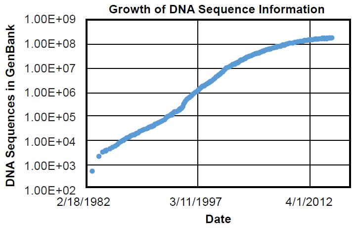
Fig. 1. Timeline of GenBank expansion. Using the data in Supplemental Table 1, the growth of the GenBank DNA sequence database was plotted over time. Massive growth in molecular information has occurred in the last few decades.
Preliminary genetic findings have already scientifically rejected Darwin’s central claims. The evolutionary answers to the questions of species’ ancestry and time of origin have failed to make accurate predictions in the realm of genetics (e.g., Bergman and Tomkins 2012; Jeanson 2013, 2015a, 2015b; Tomkins 2011, 2013a, 2013b, 2013c, 2014; Tomkins and Bergman 2012, 2015). On the question of mechanism, in 1859 Darwin’s answer may have seemed plausible, but modern molecular discoveries render it highly improbable, if not impossible, as the explanation for the origin of all life on earth (Behe 1996, 2007).
The failure of Darwinian evolution as an explanation for the origin of species does not imply that the answer to this long-standing debate is found in the species fixity model. In fact, contemporary with the revolution in genetics, the creationist model of speciation has undergone a significant advance on the questions of from whom, when, and how species originate. By carefully exegeting the text of Scripture, modern creationists have built upon and significantly modified the older explanatory framework for species origins, and they are debating a variety of mechanisms on species’ origins within the boundaries of this framework.
The first bound is the timescale in which species can arise. In contrast to evolution, the Bible permits only ~6000 years for all the diversity of life on this planet to appear (Hardy and Carter 2014). This dramatic compression of time seems, at first pass, to require unique—if not miraculous—mechanisms to explain the speciation process.
For the creation of the first ‘kinds’ during the Creation Week, miraculous activity was clearly involved. As Genesis 1 articulates, God spoke into existence the original animal ‘kinds.’ He did not derive them from one another via universal common ancestry, nor did He deistically “wind up the clock” for the universe and let the ‘kinds’ arise naturally.
At the conclusion of this Week of divine fiat activity, God ceased from creating. Since His rest from creating continues to this day (Hebrews 4:3–4) [the seventh day itself obviously does not continue to this day (Exodus 20:11)], the beginning of Day 7 marks the end of direct miraculous involvement in the origin of species.
However, after Day 7, God did not deistically forsake His creation. Rather, He providentially ruled and continues to rule His creation by “upholding all things by the word of His power” (Hebrews 1:3, NKJV) rather than by “creating new things every day by the word of His power.” He is the reason that the laws of physics and the laws of nature are in operation and continue to operate, and He is the reason that the universe hasn’t collapsed into oblivion. Though Jesus suspended some of these laws of nature and performed many miracles during His earthly ministry, and though some of His miracles seemed to involve fiat creative activity, these miracles were the exception, not the rule to God’s “upholding” activity. Hence, divine creation of new ‘kinds’ ceased after Day 6, but God’s active involvement in the universe did not—a conclusion which represents the second Scriptural bound on the origin of species question.
For Darwin’s opponents in 1859, this is where the scientific discussion largely stopped. The species’ fixity proponents of his day believed that the units of creation (the ‘kinds’) were, in fact, species, and, therefore, no new species would have formed after the Creation Week.
General Aspects of the Young-Earth Creation Speciation Model
In contrast, young-earth creation (YEC) research within the bounds of the scriptural framework has revealed that the created ‘kinds’ of Genesis 1 appear to be best approximated by the taxonomic rank of family, not species (Wood 2006, 2013). Since many families are composed of multiple species, this implies that speciation has occurred post-Creation and post-Flood. Furthermore, this fact, together with the fact of God’s continuing rest from creating, imply that these species formed via natural processes—those processes that would be classified as part of God’s “upholding” activity, such as the laws of nature, the operation of the environment, the laws of physics and chemistry, and the observable processes of genetics and cell biology.
Determining the exact number of species that have arisen via natural processes within a ‘kind’ depends on how a ‘kind’ survived the global Flood (Genesis 6–9). ‘Kinds’ that traversed the Flood outside of the Ark (e.g., fish, marine invertebrates, and probably insects and other small terrestrial invertebrates) likely did not experience as severe of a population bottleneck as the ‘kinds’ that were brought on board the Ark. Hence, several different species within each of these ‘kinds’ may have lived through the Flood. Consequently, some of the species diversity within off-Ark ‘kinds’ might be indeed due to fiat creation, implying that members of the same family may have separate ancestries while still belonging to the same ‘kind.’
If true, then explaining the origin of some species in off-Ark ‘kinds’ would not require discovering a natural mechanism.
In contrast, for those ‘kinds’ taken on board the Ark, their population sizes were reduced to two or perhaps as many as 14 individuals (Genesis 6:19–7:3), and all modern Ark-derived species have descended from these sets. Hence, for on-Ark ‘kinds,’ ‘kind’ membership is primarily a common ancestry question.
For the extant members of the terrestrial and aerial vertebrate classes (e.g., amphibians, reptiles, birds, mammals), young-earth creationists would explain the vast majority of their species diversity by processes other than fiat creation (e.g., see the number of species versus the number of families in Supplemental Table 2).2 In addition, since preliminary studies suggest that a taxonomic rank higher than family may represent the ‘kind’ boundary for some species (Lightner 2010a), the amount of speciation on the YEC timescale may be even higher. Either way, since the Flood occurred about ~4500 years ago3 (Hardy and Carter 2014), all of this diversity must have arisen in just a few thousand years.
The paleontological record adds a nuance to this statement. If we assume that the Flood/post-Flood boundary exists at the K-T (Austin et al. 1994; Whitmore and Garner 2008), then the Tertiary layers represent post-Flood burial. Since the Pleistocene layers represent Ice Age deposits, and since the Ice Age happened shortly after the Flood (Oard 1990), then Tertiary layers represent a short window of time between the end of the Flood and the ice age.
These layers contain a tremendous amount of species’ diversity, implying that a massive burst of speciation took place in just a few hundred years (Cavanaugh, Wood, and Wise 2003; Whitmore and Wise 2008; Wise 2005). For example, of the mammal families found in both the Tertiary and Quaternary layers, many more genera are preserved in the former than the latter (Table 1).4 It’s as if an enormous amount of speciation took place between the end of the Flood and the Ice Age, and then tapered off dramatically for the next several millennia. Explaining all of this diversity in just a few hundred years is the most challenging explanatory task that the YEC species’ origins model faces.
| Tertiary | Quaternary | |
|---|---|---|
| Total genera in families present in both layers | 1963 | 913 |
This burst of diversification appears to have been followed by a burst of extinction. By the time of the ice age, most of the mammalian genera that had formed as well as a similar percentage of families that were taken on board the Ark all disappeared (Table 2). Since most YE creationists put the date of the ice age in the centuries following the Flood, this period of extinction was as rapid as the proposed period of Tertiary speciation. By contrast, since the number of ice age families (Table 2) is similar to the number of extant families (see Jeanson 2015a), comparatively little extinction happened over the next several millennia.
| Tertiary | Quarternary | Total Decrease in Quaternary | Percent Decrease | |
|---|---|---|---|---|
| Total genera | 3339 | 927 | 2412 | 72 |
| Total families | 449 | 145 | 304 | 68 |
Since little overlap exists between the species found in the Tertiary and the species alive today (Table 3),5 speciation in the families that survived this extinction appears to have restarted as if the families had just exited the Ark: In the latter, genetic evidence indicates that speciation has been ongoing within ‘kinds’ at a constant rate over the last 4365 years and is even ongoing today (Jeanson 2015a). Hence, for extant species, though the timing of their origin is still short (e.g., a few thousand years), it is not as compressed as for the extinct species represented in the Tertiary layers.
| Tertiary | Extant | Extant in Tertiary (%) | |
|---|---|---|---|
| Families | 457 | 151 | 124 (82%) |
| Genera | 3339 | 1229 | 333 (27%) |
| Species | 9575 | 5436 | 135 (2%) |
Of course, if the Flood/post-Flood boundary is higher in the fossil record—perhaps at the Pliocene-Pleistocene boundary (Holt 1996)—then the most significant window of time for speciation remains a few thousand years, not a few hundred.
In short, the YEC model proposes significant amounts of morphological change in a window of time that, by comparison with evolution, is extremely short.
Despite this small temporal duration, the most relevant field to discerning the answer to the question of the mechanism of species formation is still genetics. Like Darwin, creationists hypothesize natural selection as a potential mechanism (though one of many mechanisms), and the survival of the fittest to reproduce keeps genetics at the forefront of this discussion. In addition, regardless of the role of survival in speciation, modern species are the descendants of the original creatures, and genetics will, therefore, bear the stamp of whatever mechanism gave rise to modern species.
Finally, answers to a common objection to the YEC timescale for speciation reveal additional reasons that the field most critical to fleshing out the details of how species arose is genetics. For example, opponents of YEC occasionally express serious doubt about the plausibility of producing so many species in just a few thousand years. Generating a tremendous diversity of morphologies seems, to them, an intractable problem.
Two analogies put this objection to rest and simultaneously highlight the central role of genetics in producing so many species so quickly. The first analogy comes from developmental biology. In the vast majority of metazoan species alive today, the process of development transforms a morphologically non-descript single cell into a complex, highly specialized adult form in a small window of time. For example, the wood frog (Lithobates sylvaticus) develops from a single cell to a sexually mature adult in less than three years (Herreid and Kinney 1967; see also AnAge dataset under Materials and Methods below) (Fig. 2).
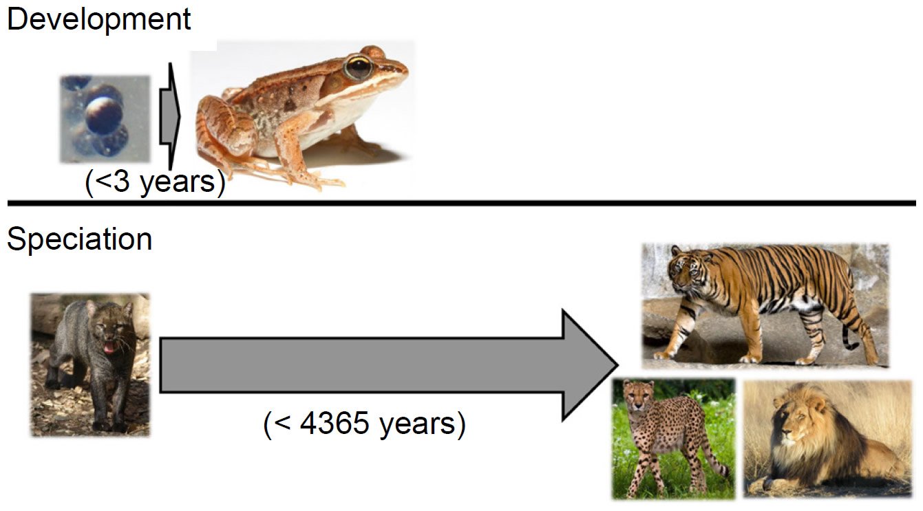
Fig. 2. Phenotypic change on various timescales. The wood frog (Lithobates sylvaticus) develops from a single cell to a sexually mature adult in less than three years, undergoing massive phenotypic transformation in the process. By contrast, over the course of 4365 years, the 37 cat species that exist today arose from a common felid ancestor—a much smaller level of phenotypic change. Thus, producing extensive phenotypic species diversity in a few thousand years is not an unreasonable postulate. Image credits: https://commons.wikimedia.org/wiki/File:Rana_sylvatica_eggs_SC.jpg. https://upload.wikimedia.org/wikipedia/commons/7/76/Lithobates_sylvaticus_%28Woodfrog%29.jpg. https://upload.wikimedia.org/wikipedia/commons/8/85/Herpailurus_yagouaroundi_Jaguarundi_ZOO_D%C4%9B%C4%8D%C3%ADn.jpg. https://upload.wikimedia.org/wikipedia/commons/e/e1/Sumatran_Tiger_Berlin_Tierpark.jpg. https://upload.wikimedia.org/wikipedia/commons/a/a9/Cheetah_5.jpg. https://upload.wikimedia.org/wikipedia/commons/7/73/Lion_waiting_in_Namibia.jpg.
In contrast, the origin of the various cat species in the family Felidae from a common ancestor on board the Ark (Pendragon and Winkler 2011) took over 4000 years. Since any two felid species have far fewer phenotypic differences between them than do an amphibian egg and an adult frog, producing a wide range of species morphologies in a few thousand years is comparatively simple. Thus, objections to the YEC timescale based on morphology alone are misguided.
Genetically, we now know that the mechanisms responsible for development are different from the mechanisms responsible for speciation. During the process of development, the zygote begins dividing, and each cell division results in the transmission of the entire genome to each daughter cell, with few exceptions (note that red blood cells in humans lack nuclei). Thus, the tremendous cell and organ diversity of the adult arises from a single cell, not via changes to the DNA sequence in each cell, but via changes in the timing and location of the expression of the DNA sequence (a.k.a. “epigenetic” changes). By contrast, millions to tens of millions of DNA sequence differences separate species from one another (e.g., see Daetwyler et al. 2014; Drosophila 12 Genomes Consortium 2007; Groenen et al. 2012; Liu et al. 2014; and many of the other recent genome sequencing papers), implying that permanent genetic changes are responsible for the origin of species, not epigenetic changes.
Nevertheless, some have still tried to argue that the mechanisms controlling these two processes are the same. For example, Dembski and Wells (2008) have suggested that DNA is not the primary physical basis for heredity, implying that analogies between development and speciation are legitimate. However, experimental data to date fail to demonstrate that epigenetic changes are stable long-term (e.g., over multiple generations), at least in animals. Instead, the primary role of epigenetics appears to be maintenance of cell identity differences within an individual, not maintenance of organismal differences between individuals (Grossniklaus et al. 2013; Heard and Martienssen 2014). Whether the data continue to trend towards this conclusion remains to be seen. Until a paradigm shift occurs, the most relevant field to consider on the question of metazoan speciation is still genetics, and if objections to the YEC timescale wish to be taken seriously, they must be based on genetics, not morphology.
The second analogy that reiterates the importance of genetics to the YEC speciation mechanism and simultaneously rebuts objections to the timescale comes from Darwin himself. His seminal publication, On the Origin of Species, opens with a comparison of breeds to species, and Darwin argued that breeds have more morphological variety among them than do some species in the wild. Though his purpose of making the analogy was directed towards the species’ ancestry question rather than the mechanism question, Darwin’s observation still holds true and is, therefore, all the more relevant today to the mechanism dispute.
For example, let the number of breeds and the number of extant species represent a measure of phenotypic diversity. In some families breeding has produced far more phenotypic diversity than speciation in the wild (Tables 4–5).6
Table 4. More breeds than species in the most domesticated mammal families.
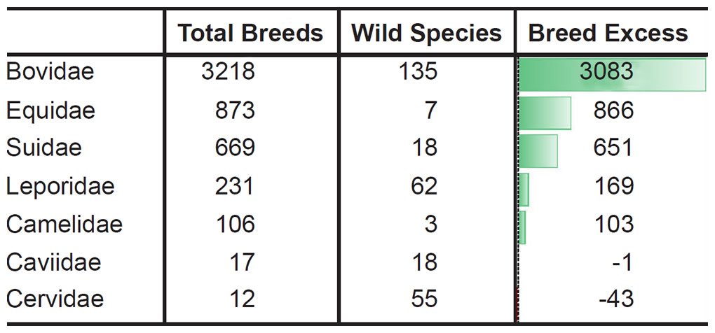
Table 5. More breeds than species in the most domesticated bird families.
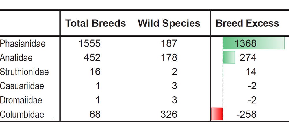
Conversely, just like species, the formation of breeds involves phenotypic change that is stable over multiple generations (Andersson 2013), implying that both are the result of genotypic type. Furthermore, since these domestic breeds arose via intelligent human intervention, these breeds must have arisen contemporary with the existence of intelligent human populations. By old-earth/evolutionary standards, intelligent human populations have been around for only a very short duration of time. Together, these facts demonstrate that a profound diversity of genetically-encoded morphologies can arise quickly, a conclusion which silences the objections to the YEC speciation timescale.
These facts also underline the importance of genetics to the YEC speciation mechanism question. If genetic change is sufficient to produce the tremendous morphological diversity in breeds, and if the morphological diversity in breeds exceeds that in species, then surely genetic change is sufficient to produce the phenotypic diversity seen in species.
Resolving the Details of the Mechanism
Within the bounds of this general speciation framework, a variety of speciation mechanisms could potentially operate. Conversely, to date, a large number of YEC hypotheses have been put forth, including directed mutation (Lightner 2009c), various forms of transposon-mediated change (Shan 2009; Terborg 2008, 2009; Wood 2002, 2003a), mediated design (Wood 2003b; Wood and Cavanaugh 2001), and fractionation of created alleles (Jeanson 2015a; Parker 1980). In the future, even more proposals might be added to this list as the number of YEC participants grows. Hence, at present, identifying which of these hypotheses—or which combination of these hypotheses—is the correct explanation remains the biggest explanatory challenge for the YEC speciation model on the question of how species originated.
Since this question is primarily historical in nature rather than a question of present processes, the weighing and evaluating of each of these hypotheses should follow several steps. First, hypotheses must be evaluated for functional relevance. For a particular speciation event, the DNA sequence(s) involved in producing the phenotypically distinct population must be identified both by knocking it (them) out to demonstrate the functional necessity of the sequence for the phenotype, and by adding it (them) back to show functional sufficiency for the species’ phenotype. Once the functionally relevant sequence(s) is (are) identified, then the various proposals on speciation mechanisms can be evaluated.
For example, one of the speciation events in the Felid ‘kind’ (Pendragon and Winkler 2011) involves the formation of stripes (e.g., in tigers). Once the DNA sequence which specifies this trait is identified, each of the YEC hypotheses on speciation should be evaluated for their ability to causally explain this relationship.
In this specific illustration, transposon-based proposals might predict transposable elements (TE) to be directly involved in the protein-coding sections of the gene(s) encoding stripes. Alternatively, transposon-based proposals might predict that TE reshuffling/insertion events would be indirectly involved—perhaps in the genomic reorganization of the nucleus such that the genes encoding stripes are transcriptionally activated. If TEs are found to have no functional relationship with the genes encoding stripes, then this hypothesis on speciation would appear functionally irrelevant on this particular speciation event/on this trait involved in speciation.
Second, hypotheses on the mechanism of speciation must be evaluated for genetic relevance. A finite number of DNA differences exist among species within a ‘kind,’ and any explanation for speciation must account for these differences.
For example, since the text of Genesis states that a minimum of two individuals and a maximum of 14 individuals went on board the Ark, a limited number of alleles at a single gene locus were present in the on-Ark ‘kinds.’ If we assume that all Ark passengers were diploid, and if we assume that only a single allele could be present at an individual gene locus, then a maximum of 28 alleles at each gene locus were carried on board this Ark (14 individuals * 2 gene copies per individual = 28 total gene copies or alleles). Today, some loci have alleles far in excess of 28 (Lightner 2008, 2009a, 2009b, 2010b), and YEC speciation models must explain the origin of these alleles.
In addition, as noted above, millions of single nucleotide variants (SNVs) separate members of the same ‘kind’ from one another. Karyotypic differences (Bedinger 2013), copy-number variants (CNVs), structural variants (SVs), and small insertion-deletions (“indels”) also exist among species within a ‘kind,’ but if humans are representative of the rest of the biological world, SNVs far outnumber all other forms of variants by an order of magnitude or more (1000 Genomes Project Consortium et al. 2015; Sudmant et al. 2015a). Nevertheless, CNVs, SVs, and indels together affect more base-pairs than SNVs. Again, a robust YEC explanation must account for the origin of all of this genetic diversity in a few thousand years
Third, hypotheses on the mechanism of speciation must be evaluated for genetic plausibility. For example, an investigator might propose that, when individuals within a ‘kind’ encounter environmental challenges, they synthesize entire biochemical systems de novo. While novel, this hypothesis is highly implausible at present—we’ve never observed this sort of phenomenon happening. No known non-miraculous mechanism exists that could play a role in this process, and invoking miracles at every juncture without biblical or scientific justification quickly moves a hypothesis from the realm of science to the realm of ad hoc speculation.
In contrast, proposals that invoke, for example, processes like transposition or random mutation are much more plausible since we have already observed the operation of these processes in the present. No miracles are required to explain these processes, and, therefore, fewer theoretical hurdles must be overcome for these hypotheses to be workable scientific explanations.
Conversely, genetic plausibility must be evaluated for each hypothesis on at least two levels. On an individual organism level, hypotheses must invoke observable processes or biblically-justified miraculous processes. At a population level, hypotheses must explain how the genetic varieties in individuals lead to the formation of populations of phenotypically distinct species. Again, observable processes or biblically-justified miraculous processes must be invoked, or the hypothesis quickly drifts into the realm of the ad hoc.
Fourth, and following naturally from the third test, hypotheses on the mechanism of speciation must be evaluated for scientific strength. Any proposed explanation for the origin of species must come in the form of a testable, predictive, accurate scientific model. Vague ideas represent good starting points for hypotheses, but a compelling scientific alternative to the evolutionary model should meet the criteria to which young-earth creationists have held evolutionists for years—namely, a match between testable expectations and actual data.
For example, creationists have long chided evolutionists for a lack of conformity between evolutionary expectations about the fossil record and the absence of bona fide transitional forms. In other instances where facts have contradicted predictions, evolutionists have waffled on their predictions, effectively demonstrating a lack of a testable hypothesis. This act has provoked further (justified) criticism from the YEC community. Conversely, young-earth creation models on the origin of species must not repeat these same errors.
Fifth, hypotheses on the mechanism of speciation must be evaluated for explanatory scope—they must explain both sides of the speciation question. As derived elsewhere (Jeanson 2013), the Flood narrative indicates that ‘kinds’ do not naturally transform into other ‘kinds,’ implying the existence of a natural biological barrier to inter-‘kind’ conversion. Hence, robust YEC explanations for the origin of a vast number of species must explain not only how genetic mechanisms produce so many phenotypes, but also how these processes did not transform one ‘kind’ into another.
For example, if directed mutations are responsible for the tremendous amount of post-Flood speciation that has occurred, why haven’t directed mutations produced a new ‘kind’ as well? What limits the adaptive creativity of directed mutations? If, instead, transposons are responsible, why haven’t transposon-mediated mechanisms produced a new ‘kind’? Similar questions could be asked of any of the YEC speciation hypotheses.
To date, little young-earth creationist investigation of the barrier to ‘kind’ transformation has been performed. While Intelligent Design advocates have identified strong barriers to Darwinian change (Behe 1996, 2007), little work has been done on the actual mechanism by which biological change is limited within the YEC view.
In this study, we attempt to advance the YEC model by articulating a testable, predictive hypothesis that we term the Created Heterozygosity and Natural Processes (CHNP) hypothesis. In short, the CHNP hypothesis is a version of the hypothesis previously referred to as the fractionation of created alleles/fractionation of heterozygosity (Jeanson 2015a; Parker 1980). Like the latter, the CHNP hypothesis proposes that diploid individuals were created heterozygous, and that natural processes since this event (including recombination, gene conversion, mutation, natural selection, etc.) have distributed and/or added to the original created genetic diversity, thus producing the genotypic and, consequently, phenotypic diversity we observe today.
To be sure, this is not a deistic hypothesis. Under the CHNP model, God doesn’t create and then abandon His creation. Rather, the CHNP model recognizes that God is actively involved in His creation, providentially upholding it to this day, and the model recognizes that God works via means, including via the environment and the natural processes that He supernaturally designed and upholds.
As an additional point of clarification, our CHNP model does not reject the operation of mutations, transposition events, or the like. Instead, we propose that ‘kinds’ started with heterozygous genomes and that the genetic variety in these genomes was modified not only by recombination and other reshuffling processes but also by mutation processes—only at rates consistent with documented genetic processes and parameters.
In other words, our model invokes a single, biblically-justified miracle of creation during the Creation Week, and then invokes observable natural processes thereafter. Thus, since our model is free of ad hoc miracles and otherwise unobservable natural processes, our model meets the first half of the criteria for the third test above, genetic plausibility at the level of the individual organism.
In the remainder of this paper, by using a variety of genetic data and population growth models, we demonstrate that our CHNP model is necessary and sufficient to account for the vast majority of eukaryotic genotypic—and, likely, phenotypic—diversity observable today. We also describe testable predictions by which our hypothesis can be further evaluated in the future. In other words, we intend to show that our model is genetically relevant, comprehensive in explanatory scope, and scientifically robust. Furthermore, in light of recent discoveries on the relationship between genotypes and phenotypes, we also argue that our model is functionally relevant.
Materials and Methods
Comparative Mitochondrial and Nuclear SNV Diversity Predictions
Analyses of mitochondrial DNA (mtDNA) were designed to match as closely as possible analyses of nuclear DNA in order to make the comparisons between the two compartments as parallel as possible. Consequently, some of the mtDNA analyses published previously (Jeanson 2015a) were updated to more closely mirror the nuclear DNA analyses performed in this study.
For humans, nuclear single nucleotide variant (SNV) analyses were performed on non-Africans as a group (see below). Hence, in this study, human mtDNA SNV analyses were copied directly from those published previously (Jeanson 2015b) without further modification.
In Drosophila, nuclear SNV analyses were performed only on D. melanogaster and D. simulans. Therefore, we used their mtDNA NCBI accession numbers (same as those in the previously published Drosophila mtDNA analyses [Jeanson 2015a]) to obtain their whole mtDNA genome sequences from NCBI Nucleotide (http://www.ncbi.nlm.nih.gov/nuccore), and these sequences were aligned with CLUSTALX 2.1 (http://www.clustal.org/clustal2/). The resultant alignment file was imported into BioEdit (http://www.mbio.ncsu.edu/bioedit/bioedit.html), and all non-standard nucleotide sequences (e.g., N, M, R, Y, B, W, S, V, H, D) were replaced with gaps. Then all gaps were stripped from the alignment. BioEdit was then used to create a sequence difference count matrix, which identified 634 mtDNA differences between the two species. This number was compared to the mtDNA SNV mutation rate predictions published previously (Jeanson 2015a).
For Daphnia pulex, nuclear SNV predictions were compared to an estimate of the range of nuclear SNV differences among several individuals in the same species. Hence, the previously published D. pulex mtDNA SNV predictions were copied directly from those published previously (Jeanson 2015a) without further modification, and mtDNA mutation rates were copied directly from those published previously (Jeanson 2015a) without further modification. However, these predictions were compared to a range of mtDNA SNV differences among several D. pulex individuals, and these numbers were extracted from mtDNA alignments performed previously (see Jeanson 2015a for methods; see Supplemental Table 5 for pairwise DNA differences).
For the Saccharomyces cerevisiae mtDNA analyses, mtDNA SNV diversity was predicted using the divergence calculation published previously (Jeanson 2015a). In short, the empirically derived whole mtDNA genome mutation rate (Lynch et al. 2008) in units of mutations/base-pair/generation was converted to a rate in units of mutations/mtDNA genome/year using a published range of generation times for S. cerevisiae (Herskowitz 1998) and an approximation of the range of mtDNA genome sizes for S. cerevisiae from NCBI (http://www.ncbi.nlm.nih.gov/genome/browse/). This converted rate was used to predict how many base-pair differences would arise in 6000 years (e.g., rate * 6000 * 2 = predicted diversity) (see Supplemental Table 6 for details of the calculations).
This prediction was compared to an estimate of the mtDNA SNV differences between S. cerevisiae and one of its closest relatives (Kellis et al. 2003), S. paradoxus. Since significant mtDNA genomic structural differences exist between S. cerevisiae and S. paradoxus, a simple pair-wise whole mtDNA genome alignment between the two species was not possible. Instead, the nucleotide divergence between the two genomes was estimated from a gene-by-gene comparison of the two genomes published previously (Procházka et al. 2012). The average nucleotide divergence for these regions was multiplied by an approximation of the range of mtDNA genome sizes for S. cerevisiae from NCBI (http://www.ncbi.nlm.nih.gov/genome/browse/) (see Supplemental Table 6 for details of the calculations).
Nuclear DNA comparisons for all four species were performed according to a common protocol. First, nuclear SNV mutation rates were obtained from the published literature (Conrad et al. 2011 for Homo sapiens; Haag-Liautard et al. 2007; Keightley et al. 2014 for Drosophila melanogaster; Lynch et al. 2008; Zhu et al. 2014 for Saccharomyces cerevisiae; and Keith et al. 2016 for Daphnia pulex).
Second, these published rates were converted to more useful units. The published rates were measured in units of mutations/base-pair/generation, and they were converted to mutations/genome/year with the generation times and genome sizes for each species. Generation times were estimated for humans to be between 15 and 35 years, and generation times were obtained from the literature or from academic websites for Drosophila melanogaster (Jeanson 2015a), Saccharomyces cerevisiae (Herskowitz 1998), and Daphnia pulex (Jeanson 2015a). Nuclear genome sizes for each of these species were obtained from NCBI (http://www.ncbi.nlm.nih.gov/genome/browse/).
Because all four species possess a diploid stage during at least part of their life cycle, the nuclear DNA mutation rates were multiplied by 2 to determine the mutation rate in units of mutations/diploid genome/year.
Third, the converted mutation rates were used to predict genetic diversity over 6000 years for these species (see Supplemental Table 6 for details of the calculations). To capture the full statistical spectrum of predictions, the highest and lowest measures of the published rate (e.g., standard error, standard deviation, etc.) were matched with the fastest and slowest (respectively) generation times for each species.
In most cases, our predictions were for nucleotide differences between separate species, and we used a divergence equation (rate * time * 2 = nucleotide differences) for this purpose. Since the human individuals were from the same species and since the Daphnia pulex individuals were all from the same species, we used a coalescence calculation (rate * time = nucleotide differences) to make our predictions.
Fourth, these predictions were compared to measures of actual nuclear DNA diversity within or between species. In Homo sapiens, the range of heterozygosity estimates for individuals from several different non-African ethnic groups (Table 1 of Kim et al. 2014) was multiplied by the genome size for humans (http://www.ncbi.nlm.nih.gov/genome/browse/) to determine absolute DNA differences (see Supplemental Table 6 for calculations).
Among Drosophila species, several possessed published nuclear diversity data (Begun et al. 2007; Garrigan et al. 2012, 2014; Richards et al. 2005). We used D. simulans for the comparison, and we multiplied the estimate of the divergence between D. simulans (Garrigan et al. 2012) and D. melanogaster by the D. melanogaster nuclear genome size (http://www.ncbi.nlm.nih.gov/genome/browse/) to obtain the actual nucleotide difference between these two species (see Supplemental Table 6 for calculations).
Nuclear DNA diversity predictions for Daphnia pulex were compared to the range of heterozygosity estimates from multiple D. pulex individuals (see Fig. 1 of Tucker et al. 2013).
Nuclear DNA diversity predictions for Saccharomyces were compared to an estimate of the genomic divergence between S. cerevisiae and S. paradoxus (Kellis et al. 2003), the closest S. cerevisiae relative that possesses a published nuclear genome sequence. The average percent identity in the protein-coding regions of the genome was higher than the average percent identity in the intergenic regions. Since ~70% of the S. cerevisiae genome consists of genic sequence (Goffeau et al. 1996), we multiplied the coding region identity by 0.7 and the intergenic region identity by 0.3, and then added the totals together to obtain an estimate of the genome-wide nucleotide divergence between the two species (see Supplemental Table 6 for calculations).
Human Rare Variant Predictions
The nuclear DNA mutation rate for Homo sapiens was obtained from the published literature (Conrad et al. 2011). Since this rate was measured in units of mutations/base-pair/generation, it was converted to units of mutations/diploid genome/year with the generation times estimated to be between 15 and 35 years. The haploid nuclear genome size for humans was obtained from NCBI (http://www.ncbi.nlm.nih.gov/genome/browse/).
This converted rate was used to predict the number of rare variants that would arise in each individual since the Flood. Since all individuals alive today genetically descend from three couples on board the Ark (Genesis 9:18–19), nuclear DNA variants that were present in Shem, Ham, and Japheth and in their wives likely would be well distributed around the world today. It’s only after these couples started reproducing and after the human population began to explosively recover in size that new mutationally-derived alleles would have been poorly distributed around the globe. Hence, the converted nuclear DNA mutation rate was multiplied by 4365 years (the Flood date) rather than 6000 years (the Creation date).
Multiplying the mutation rate and the time (representing a coalescence calculation), we predicted the number of rare variants present today in each individual (see Supplemental Table 6 for the details of these calculations), and these predictions were compared to the published per-individual count of rare alleles, defined as a derived allele frequency <0.5% (see Table S14 of 1000 Genomes Project Consortium et al. 2012). Since Africans appear to recombine DNA faster than non-Africans (Hinch et al. 2011), and since this fact could move variants from the common or intermediate variant categories to the rare category preferentially in Africans, we compared our predictions to the number of rare variants only in non-Africans.
Human Haplotype Block Predictions
Adam and Eve were assumed to have been created with nuclear DNA heterozygosity, implying that their genomes represented the first haplotype blocks. Since they were the only individuals alive, their “haplotype blocks” were, essentially, the length of entire chromosomes. Therefore, every recombination and gene conversion event since the creation of their genomes would fragment these initially long blocks into smaller haplotype blocks.
To predict how many blocks would have arisen in each individual after 6000 years, the published rate of recombination (Wang et al. 2012) and several estimates of the frequency of gene conversion (Palamara et al. 2015; Wang et al. 2012; Williams et al. 2015) were combined into a total rate of haplotype block division per generation. For the gene conversion rate, Wang et al. (2012) estimated about 250–800 gene conversion events per cell, and Williams et al. (2015) estimated 228 from a per nucleotide rate that was the same as the per nucleotide rate reported in Palamara et al. (2015). We used 220 gene conversion events per cell in our calculations.
The combined gene conversion and recombination rate was divided by a range of generation time estimates for humans (35 years to 15 years) to determine the rate of haplotype block divisions per year. Multiplying this converted rate by 6000 years estimated the number of haplotype blocks that would have resulted from 6000 years of recombination and gene conversion in each generation in a single lineage (see Supplemental Table 6 for details of these calculations).
These predictions were compared to the current number of haplotype blocks, estimated via linkage disequilibrium to be 5,400 nucleotides (Rosenfeld, Mason, and Smith 2012). Dividing this block size into the human haploid genome size (http://www.ncbi.nlm.nih.gov/genome/browse/), we determined the average number of total blocks in the human genome. Since the reported haplotype block number was derived via comparison of 90 individuals, we modified our haplotype block predictions to estimate the number of blocks that would result from the comparison of several lineages. With just seven lineages, our predictions easily captured the current number of total blocks in the human genome (see Supplemental Table 6 for details of these calculations).
Assessment of the Relationship between Nuclear Heterozygosity and Nuclear Mutation Rates
In Arabidopsis, the relationship between nuclear SNV mutation rates and nuclear heterozygosity was previously published on a relative scale with respect to heterozygosity (e.g., see the x-axis of Figure 2b of Yang et al. 2015). We converted the x-axis (heterozygosity) to an absolute scale via the following steps: (1) The Col-Ler whole genome strain difference (e.g., by definition, this represented the heterozygosity of the F1 parents in the F1 →F2 measurement since Col and Ler were crossed to generate F1 progeny) was estimated from the dashed blue line in Fig. 2d of Yang et al. (2015) to be about 0.0038 (0.38%). (2) Since 0.0038 represented the “1.0” value on the relative heterozygosity scale in the graph of Fig. 2b of Yang et al. (2015), and since this same graph represented the heterozygosity of the parents in the F2 →F3 measurements and F3→F4 measurements as “0.5” and “0.25” (due to the fact that reproduction was induced via selfing, which decreases heterozygosity by half in each generation that it is performed), respectively, we assigned values of 0.0019 (e.g., 0.0038/2) and 0.00095 (e.g., 0.0019/2), respectively, to these positions on the graph. Based on the display in Fig. 2d of Yang et al. (2015), we set the heterozygosity of the P0→P1 measurements to zero.
We also plotted the mutation rate and heterozygosity values from four species on this same absolute scale graph. The SNV mutation rate values were obtained from the literature for Homo sapiens (Conrad et al. 2011), Drosophila melanogaster (Haag-Liautard et al. 2007; Keightley et al. 2014), Saccharomyces cerevisiae (Lynch et al. 2008; Zhu et al. 2014), and Daphnia pulex (Keith et al. 2016).
For absolute heterozygosity values, the human heterozygosity values across ethnic groups was obtained from the published literature (see Table 1 of Kim et al. 2014). For the two papers from which we obtained the nuclear DNA mutation rate for Drosophila melanogaster, one paper (Haag-Liautard et al. 2007) reported using sibling matings/inbreeding for the experiment, and the other paper (Keightley et al. 2014) reported using individuals from isofemale lines. In light of these facts and in light of the fact that Drosophila males do not undergo recombination, we treated the heterozygosity value as inbred and set it to zero.
For D. pulex, the nuclear DNA mutation rate paper (Keith et al. 2016) indicated that heterozygosity in the individuals analyzed was similar to heterozygosity in reported in a previous publication (Tucker et al. 2013). We used the lower end of the heterozygosity values (e.g. 0.01) reported in Fig. 1 of Tucker et al. (2013).
The yeast publications (Lynch et al. 2008; Zhu et al. 2014) describing the measurement of the nuclear DNA mutation rate used either nearly completely homozygous or haploid strains. Thus, we set the heterozygosity value to zero.
For all four of these species, the published ranges or statistical errors associated with the measurements of heterozygosity, and/or the published ranges or statistical errors of the nuclear SNV mutation rate were reflected in the error bars in our plots.
Raw values supporting the discussion in this section were deposited in Supplemental Table 7.
Plant Nuclear DNA Mutation Rate Predictions
In light of the positive relationship between nuclear DNA heterozygosity and nuclear DNA mutation rates in Arabidopsis thaliana (Yang et al. 2015), we predicted mutationally-derived SNVs on the YEC timescale. To model a state of no pre-existing heterozygosity (e.g., not the CHNP model), we used the lowest reported nuclear DNA mutation rate in Yang et al. (2015) to predict mutation-derived DNA diversity on the YEC timescale. As per the protocol above, this mutation rate was converted from units of mutations/base-pair/generation to mutations/genome/year with the generation time from the literature for Arabidopsis thaliana (Ochatt and Sangwan 2008) and with the genome size from NCBI (http://www.ncbi.nlm.nih.gov/genome/browse/). Since A. thaliana is diploid, the nuclear DNA mutation rate was multiplied by 2 to determine the mutation rate in units of mutations/diploid genome/year.
This converted mutation rate was used to predict genetic diversity over 6000 years (see Supplemental Table 6 for details of the calculations). Since our predictions were for nucleotide differences between separate species (see below), we used a divergence equation (rate * time * 2 = nucleotide differences) for this purpose.
Our predictions were compared to measures of actual nuclear DNA diversity between Arabidopsis species (Hu et al. 2011). The number of SNV differences between A. thaliana and A. lyrata was obtained directly from Fig. 1d (e.g., the alignable mismatches) of Hu et al. (2011).
Additional Nuclear SNV Mutation Rate Predictions
To ascertain whether a relationship between nuclear SNV heterozygosity and nuclear SNV mutation rates existed in other species, we obtained the mutation rates from the published literature for Pan troglodytes (Venn et al. 2014), Mus musculus (Uchimura et al. 2015), Heliconius melpomene (Keightley et al. 2015), Apis mellifera (Yang et al. 2015), Chlamydomonas reinhardtii (Ness et al. 2012, 2015), and Schizosaccharomyces pombe (Farlow et al. 2015).
To estimate the heterozygosity in Pan troglodytes, the heterozygosity within Western chimpanzees (Fig. 1b of Prado-Martinez et al. 2013) was used as a surrogate for the heterozygosity in the individuals used for the mutation rate measurement.
Since the individuals used to measure the mutation rate in Mus musculus were highly inbred and in Heliconius melpomene were partially inbred, we set their heterozygosity levels to zero. In at least one of the Chlamydomonas reinhardtii mutation accumulation experiments (Ness et al. 2012), the authors explicitly used asexually reproducing (e.g., effectively haploid) individuals. We used the mutation rate from only this experiment, and we set the C. reinhardtii heterozygosity to zero. In the Schizosaccharomyces pombe experiment, the lines were maintained as haploid, and the heterozygosity was, therefore, set to zero.
For Apis mellifera, the average number of heterozygous sites was calculated from Table S2 of Liu et al. (2015), and this number was divided into the A. mellifera genome size (http://www.ncbi.nlm.nih.gov/genome/browse/).
From these mutation rates and heterozygosity estimates, we plotted data points by overlaying the information from each species on the Arabidopsis graph that relates nuclear SNV heterozygosity and nuclear SNV mutation rates (description of graph in a previous section).
For all six of these species, the published ranges or statistical errors associated with the measurements of heterozygosity, and/or the published ranges or statistical errors of the nuclear SNV mutation rate were reflected in the error bars in our plots.
Raw values supporting the discussion in this section were deposited in Supplemental Table 7.
Then nuclear SNV predictions for these six species were performed, and we used a common protocol for all six species. First, the published mutation rates were converted from units of mutations/base-pair/generation to mutations/genome/year with the generation times and genome sizes for each species.Generation times were obtained from the literature or from academic websites for Pan troglodytes (Table 1 of Langergraber et al. 2012; only Western chimpanzee data were used), Mus musculus (http://www.informatics.jax.org/silver/chapters/1-3.shtml; I also used the six week generation time that I observed on occasion in C57Bl/6 mice during my graduate school experience), Heliconius melpomene (Kronforst 2008; Pardo-Diaz et al. 2012), Apis mellifera (Wallberg et al. 2014), Chlamydomonas reinhardtii (Harris 2001), and Schizosaccharomyces pombe (http://research.stowers.org/baumannlab/documents/Nurselab_fissionyeasthandbook_000.pdf). Nuclear genome sizes for each of these species were obtained from NCBI (http://www.ncbi.nlm.nih.gov/genome/browse/) or from the publications from which nuclear SNV diversity was obtained (see below).
Since all six species exist in the diploid state for at least part of their life cycle, the nuclear SNV mutation rates were multiplied by 2 to determine the mutation rate in units of mutations/diploid genome/year.
Second, these converted mutation rates were used to predict genetic diversity over 6000 years. If predictions were compared to SNV differences within the species, a coalescence calculation (diversity = mutation rate * time) was used. When predictions were compared to SNV differences between species, a divergence equation (diversity = mutation rate * time * 2) was used. To capture the full statistical spectrum of predictions, the highest and lowest measures of the published rate (e.g., standard error, standard deviation, etc.) were matched with the fastest and slowest (respectively) generation times for each species.
Third, these predictions were compared to measures of actual nuclear SNV diversity between species. Pan troglodytes nuclear SNV diversity predictions were compared to the SNV diversity within the species (Table 1 of Prado-Martinez et al. 2013). We selected the highest mean SNV per individual value among the values listed for the various Pan troglodytes subspecies.
Mus musculus nuclear SNV diversity predictions were compared to the number of SNV differences between the C57Bl/6 strain and a strain (SPRET/EiJ) derived from Mus spretus (Table 1 of Keane et al. 2011).
Heliconius melpomene nuclear SNV diversity predictions were compared to the number of SNV differences between H. melpomene and H. hecale (Table S2 of Kronforst et al. 2013).
Apis mellifera nuclear SNV diversity predictions were compared to the number of SNV differences among Apis mellifera subspecies (Table 1 of Wallberg et al. 2014). The highest SNV number was chosen for comparisons.
Since no genomic SNV comparisons were available for inter-species comparisons within the genus Chlamydomonas, we used the highest published intra-species SNV difference for C. reinhardtii (Flowers et al. 2015).
Since no genomic SNV comparisons were available for inter-species comparisons within the genus Schizosaccharomyces, we used the average pairwise SNV diversity among S. pombe strains (Jeffares et al. 2015).
See Supplemental Table 6 for details of these calculations.
Insertion-Deletion (Indel) and Copy-Number Variant (CNV) Predictions
Mutational predictions of insertion-deletion variants (indels) and copy-number variants (CNV) were made for four species. The human insertion-deletion (indel) mutation rate [for indels 20 base-pairs or less in length] and large structural variant (SV) mutation rate [this included deletions and insertions larger than 20 base-pairs, as well as duplications, and retrotranspositions] were obtained from the literature (Kloosterman et al. 2015). Since our comparisons below were to indels that appeared to be 50 base-pairs long or less, and since the reported rate was for indels ≤20 base-pairs and for structural variants >20 base-pairs, we lumped the indel mutation rate (2.94 per generation) together with the SV mutation rate (0.16). We predicted the number of indels that would result via a constant mutation rate over 6000 years using a range of generation time estimates (15 years to 35 years) and using a coalescence equation (indels = mutation rate * time). These predictions were compared to the lowest number of reported indels per individual, as well as to other types of non-SNVs per individual (see Table 1 of 1000 Genomes Project Consortium et al. 2015 and Table 1 of Sudmant et al. 2015b).
For Arabidopsis, the indel mutation rate for indels 1- to 3- base-pairs in length was obtained from the published literature (Ossowski et al. 2010). The mutation rate was converted from units of mutations/site/generation to units of mutations/genome/year using generation times as in previous sections and the nuclear genome size for Arabidopsis thaliana as in previous sections, and it was multiplied by 2 to convert it to units of mutations/diploid genome/year. Then the indel divergence between two Arabidopsis species over 6000 years was calculated via a divergence equation (divergence = mutation rate * time *2). This prediction was compared to divergence in terms of 1 to 3 base-pair indels between A. thaliana and A. lyrata (see Fig. 2 of Hu et al. 2011). The latter was determined by adding together the 1, 2, or 3 base-pair indels that were missing (“deleted”) in either species.
For Mus musculus, the indel mutation rate was obtained from the published literature (Uchimura et al. 2015). The mutation rate was converted from units of mutations/site/generation to units of mutations/genome/year using generation times as in previous sections and the nuclear genome size for Mus musculus as in previous sections, and it was multiplied by 2 to convert it to units of mutations/diploid genome/year. Then the indel divergence between two mouse species over 6000 years was calculated via a divergence equation (divergence = mutation rate * time *2). This prediction was compared to indel divergence between the C57Bl/6 strain and the SPRET/EiJ strain (derived from Mus spretus) (Keane et al. 2011).
For Drosophila, the indel mutation rates were obtained from the published literature (Haag-Liautard et al. 2007; Schrider et al. 2013). The mutation rate was converted from units of mutations/site/generation to units of mutations/genome/year using generation times as in previous sections and the nuclear genome size for Drosophila melanogaster as in previous sections, and it was multiplied by 2 to convert it to units of mutations/diploid genome/year. Then the indel divergence between two Drosophila species over 6000 years was calculated via a divergence equation (divergence = mutation rate * time *2). This prediction was compared to the indel divergence between D. melanogaster and D. simulans (see Table S1 of Begun et al. 2007) by adding the pairwise autosome diversity (π) for insertions to that for deletions, and then multiplying this by the D. melanogaster genome size (http://www.ncbi.nlm.nih.gov/genome/browse/).
See Supplemental Table 6 for details of these calculations.
Measurement of Historical Changes in SNV Heterozygosity
Historical changes in SNV heterozygosity levels were scored for diverse species and biological families according to a common protocol. First, species with measured SNV levels between individuals of different species and SNV heterozygosity levels within the same individual of a species were identified for various families.
Second, the most distant pairwise SNV levels were identified among the available species within a family. This value was used to represent the putative SNV heterozygosity levels in the ‘kind’ ancestor of the modern species within the family. Obviously, since we sampled only a few species within a family, under the CHNP model this likely represented an underestimate of the SNV levels in the ‘kind’ ancestor.
Third, the SNV heterozygosity levels in modern species were compared to the calculated SNV heterozygosity in the ancestor, and the fold-drop was scored between the two values.
For Drosophila melanogaster, the SNV difference between D. melanogaster and D. sechellia (Garrigan et al. 2012) was used to simulate the heterozygosity of the Drosophilid ‘kind’ ancestor. Heterozygosity in modern D. melanogaster species was more difficult to obtain due to idiosyncrasies of the isolation and sequencing protocols (e.g., wild individuals were often obtained and then inbred before sequencing, effectively making measurement of heterozygosity in the wild impossible). In lieu of this challenge, we used the highest reported value from a comparison of SNVs between individuals in the D. melanogaster species (Fig. 2 of Pool et al. 2012) as an estimate of what the heterozygosity in individual flies in the wild might be. Presumably, some of these SNVs represent homozygous variants; therefore, our number represents an upper bound and likely overestimate of current levels of heterozygosity in individual flies in the wild.
For Arabidopsis thaliana, we performed a similar type of comparison. The SNV difference between A. thaliana and A. lyrata (Supplementary Fig. 1a of Hu et al. 2011) was used to simulate the heterozygosity of the Arabidopsis ‘kind’ ancestor. Heterozygosity in modern A. thaliana individuals was estimated by taking the average of the SNV differences between individuals in the A. thaliana species (Supplementary Table 1 of Cao et al. 2011) and dividing it by the A. thaliana genome size (http://www.ncbi.nlm.nih.gov/genome/browse/). Presumably, some of these SNVs represent homozygous variants; therefore, our number represents an upper bound and likely overestimate of current levels of heterozygosity in individual A. thaliana plants in the wild.
For Macaca comparisons, we divided the maximum SNV difference between M. fascicularis and M. mulatta (Supplementary Table 8 of Yan et al. 2011) by the reported genome size of M. fascicularis (Yan et al. 2011) to simulate the heterozygosity of the Cercopithecidae ‘kind’ ancestor. Heterozygosity in modern M. mulatta and M. fascicularis was reported in Supplementary Table 8 of Yan et al. (2011).
For comparisons in the Suidae family, we divided the SNV difference between Sus scrofa and Phacochoerus africanus (Supplementary Table 18 of Groenen et al. 2012) by the reported S. scrofa genome size (Groenen et al. 2012) to simulate the heterozygosity of the Suid ‘kind’ ancestor. Heterozygosity for wild pigs and P. africanus was calculated by dividing the number of reported heterozygous sites in Supplementary Table 18 of Groenen et al. (2012) by the reported S. scrofa genome size (Groenen et al. 2012). Since there were four wild pigs with reported heterozygous sites, we took the average of the four individuals.
For Bos mutus, we divided the SNV difference between B. frontalis and B. taurus (Table 2 of Mei et al. 2016) by the B. taurus genome size (http://www.ncbi.nlm.nih.gov/genome/browse/) to simulate the heterozygosity of the Bovinae ancestor of the modern Bos species. Heterozygosity for B. mutus was reported in Table S1 of Wang et al. (2014).
For Capra aegagrus, we multiplied the O. aries genome size (http://www.ncbi.nlm.nih.gov/genome/browse/) by the percent of the genome (95%) that the O. canadensis alignment covered. We then divided the SNV difference between Ovis canadensis and O. aries (Miller et al. 2015) into this modified genome size number in order to simulate the heterozygosity of the Caprinae ancestor of the modern Capra and Ovis species. Heterozygosity for C. aegagrus was reported in Dong et al. (2015).
For species in the family Felidae, we divided the SNV difference between Panthera tigris and Felis catus (Supplementary Table S15 of Cho et al. 2013) by the F. catus genome size (http://www.ncbi.nlm.nih.gov/genome/browse/) to simulate the heterozygosity of the Felid ‘kind’ ancestor. Heterozygosity for P. tigris, P. leo, and P. uncia was reported in Supplementary Table S57 of Cho et al. (2013) (if two values were reported for the same species, the average was taken), and heterozygosity for Acinonyx jubatus was obtained by taking the average of the heterozygosity values for A. jubatus individuals reported in Table S20 of Dobrynin et al. (2015).
For species in the family Balaenopteridae, we divided the SNV difference between Balaenoptera physalus and B. acutorostrata (Supplementary Table 56 of Yim et al. 2014) by the genome size of B. acutorostrata (http://www.ncbi.nlm.nih.gov/genome/browse/) to simulate the heterozygosity of the Balaenopteridae ‘kind’ ancestor. Heterozygosity values for these two species were obtained from Supplementary Table 56 of Yim et al. (2014).
For species in the family Spheniscidae, we obtained the SNV difference between Pygoscelis adeliae and Aptenodytes forsteri from p. 9 of Li et al. (2014) where the authors reported 79,551,994 SNV differences over an aligned sequence length of 1,066,586,108. The heterozygosity values for these species were obtained from p. 2 where the reported number of heterozygous sites for each species was divided into the reported genome size (without gap sequence) for each species.
Measurement of Historical Changes in Indel Heterozygosity
Historical changes in indel heterozygosity levels were scored for a single Felid species. We divided the indel difference between Panthera tigris and Felis catus (Supplementary Table S15 of Cho et al. 2013) by the F. catus genome size (http://www.ncbi.nlm.nih.gov/genome/browse/) to simulate the indel heterozygosity of the Felid ‘kind’ ancestor. Heterozygous indels in P. tigris were reported in Supplementary Table S15 of Cho et al. (2013), and we divided this value by the P. tigris genome size (http://www.ncbi.nlm.nih.gov/genome/browse/) to derive the indel heterozygosity value in P. tigris today. The fold-drop was scored between the ancestor and modern P. tigris values.
Population Growth Calculations
The AnAge dataset was downloaded from the Ageing Database (http://genomics.senescence.info/species/) on March 6, 2015. The acceptable and high quality data for species in Mammalia were extracted by sorting the dataset by “Class” designation and keeping only the rows with a “Mammalia” designation. Then the data were sorted by “Female maturity (days)”, and all rows with blank entries in this column were removed. Then the data were sorted by “Male maturity (days)”, and all rows with blank entries in this column were removed. Then the data were sorted by “Gestation/Incubation (days)”, and all rows with blank entries in this column were removed. Then the data were sorted by “Weaning (days)”, and all rows with blank entries in this column were removed. Then the data were sorted by “Litters/Clutches per year”, and all rows with blank entries in this column were removed. Then the data were sorted by “Maximum longevity (yrs)”, and all rows with blank entries in this column were removed. Then the data were sorted by “Data quality”, and all rows with “questionable” designations in this column were removed. This process of data curation resulted in a final dataset consisting of 363 mammalian species with known growth rate parameters (Supplemental Table 8).
Population growth equations were calculated by computer simulation. Since unconstrained population growth is proportional to the number of living, reproducing organisms, growth curves are an exponential function of time. Therefore, after the first several generations, the total unconstrained population of any species as a function of time can be expressed as Aeλt, where e is Euler’s number (approximately 2.71828), t is the time (in years), and A and λ are constants that will depend on reproductive parameters (such as lifespan and litter size) and will therefore differ from species to species. To compute A and λ for each species, we simulated the population growth based on the parameters of that species, keeping track of the total number of individuals at each step.
Starting from two initial organisms of the selected species, we track the total number of individuals at each time step, where the time step is selected to be the inverse of the average number of litters per year. At each time step, the population is increased by the average litter size of the species multiplied by the number of extant reproducing pairs. We assume an equal number of males and females, and thus the number of reproducing pairs is taken to be half the number of reproductively mature individuals. At any given time step, the simulation separately tracks both non-reproducing and reproducing individuals, and moves those from the former bin into the latter bin once they reach sexual maturity. When any individual reaches or exceeds the average lifespan of its species, it is removed from the population and no longer counted.
This is done for 40 time steps to build a statistically significant curve separately for each species. We then compute the best-fit exponential function for each curve, which gives the coefficient (A) and growth constant (λ) for each species. From these parameters, we can compute the expected unconstrained population of any species at any time t.
Taxonomic Designations
The common names for various species and taxonomic designations used in this study is available in Supplemental Table 9.
Results and Discussion
(A) Testing the genetic relevance and scientific strength of the CHNP model
(1) The origin of SNVs
(a) Mitochondrial “clocks” contradict nuclear DNA “clocks”
The recent discovery of a mitochondrial single nucleotide variant (SNV) “clock” that measures time consistent with the YEC timescale (Jeanson 2013, 2015a, 2015b) suggested an arena by which the origin of SNV diversity among species could be interrogated. These previous studies demonstrated strong agreement between the predictions of a 6,000-year, constant-rate mutational clock and actual measures of genetic diversity, and this finding was true across metazoan phyla (Figs. 3A, 4A, 5A). (Since the purpose of showing these mtDNA data was to eventually compare them to nuclear SNV data, we omitted the previously published Caenorhabditis mtDNA results for lack of appropriate nuclear SNV comparisons among Caenorhabditis species.)
We extended these mtDNA studies by making predictions for yeast using the empirically-derived SNV mutation rates, and we found similar agreement between predictions and extant diversity (Fig. 6A). In fact, the current rate of mtDNA change predicted a maximum DNA difference in excess of the yeast mtDNA genome size.
Since we used the yeast generation time observed in the laboratory under ideal conditions, the doubling time of yeast might be slower in the wild, which would bring the maximum predicted DNA difference value below the mtDNA genome size. Regardless, these results demonstrated the sufficiency of constant mutation rates to explain mitochondrial SNV sequence diversity on the YEC timescale. Hence, mitochondrial SNV clocks appeared to exist across major kingdoms of life.
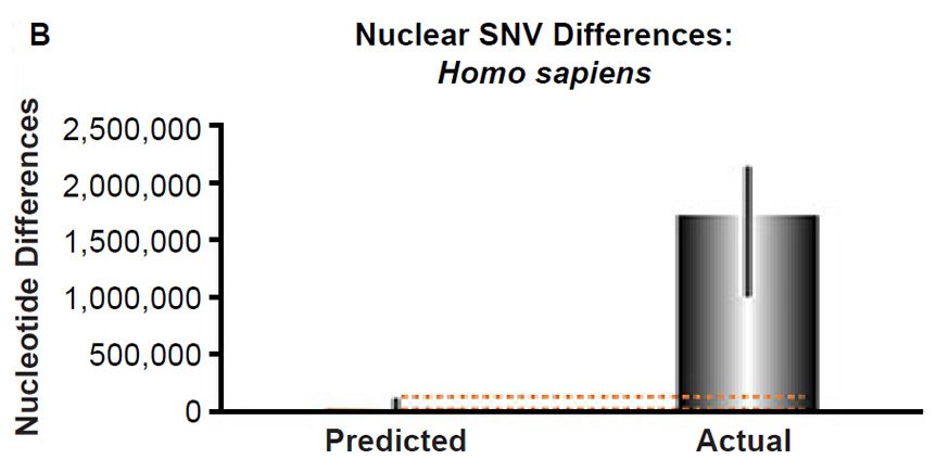
These four species with mtDNA SNV clocks also happened to have published nuclear SNV mutation rates. Using the same assumption of constant mutation rates that we employed for mtDNA predictions, nuclear SNV diversity predictions were made for all four of these species, but all four predictions severely underestimated existing nuclear SNV diversity (Figs. 3B, 4B, 5B, 6B). In fact, for three of the species (Figs. 3B–5B), the average prediction underestimated the average actual diversity by nearly an order of magnitude or more. Thus, whether we investigated humans, animals, or fungi, >75% of the nuclear SNV diversity was inexplicable via a constant rate of random mutations over time, and our results strongly rejected the hypothesis of whole genome nuclear SNV clock.
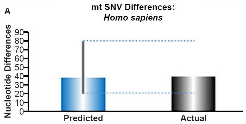
(A) Using the measured SNV mutation rate for the whole mitochondrial DNA (mtDNA) genome in non-African people groups, the number of mtDNA SNV differences was predicted assuming a constant rate of DNA change over 6000 years. This prediction was compared to the current levels of mtDNA SNV differences in non-African people groups. The height of each bar represented the average DNA difference, and the thick black lines represented the range of predicted values given the reported error in the mutation rate and given the range of generation time estimates (“Predicted” bar). As the dotted lines demonstrate, the predicted number of differences overlapped the current differences among non-Africans. Adapted from Fig. 1 of Jeanson (2015b).
(B) Using the measured SNV mutation rate for the whole nuclear DNA genome in humans, the number of SNV differences was predicted assuming a constant rate of DNA change over 6000 years. This prediction was compared to heterozygosity estimates for individuals from several different non-African ethnic groups. The height of each bar represented the average DNA difference, and the thick black lines represented the range of predicted values given the reported error in the mutation rate and given the range of generation time estimates (“Predicted” bar). For the “Actual” bar, the thick black lines represented the current range of reported nuclear DNA differences among non-African groups. As the dotted lines demonstrate, predictions clearly underestimated actual differences.
Fig. 3. Contradiction between mtDNA and nuclear DNA SNV clocks in humans.
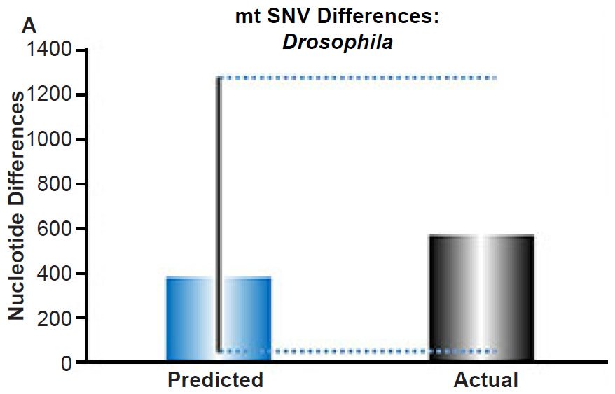
(A) Using the measured SNV mutation rate for the whole mitochondrial DNA (mtDNA) genome in Drosophila melanogaster, the number of SNV differences was predicted assuming a constant rate of DNA change over 6000 years. This prediction was compared to the current levels of mtDNA SNV differences between D. melanogaster and D. simulans. The height of each bar represented the average DNA difference, and the thick black lines represented the range of predicted values given the reported error in the mutation rate and given the range of generation time estimates (“Predicted” bar). As the dotted lines demonstrate, the predicted number of differences captured the current levels of mtDNA differences between these two species. Adapted from Fig. 9 of Jeanson (2015a).
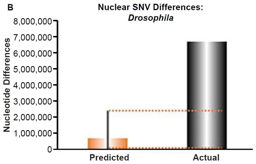
(B) Using the measured SNV mutation rate for the whole nuclear DNA genome in Drosophila melanogaster, the number of SNV differences was predicted assuming a constant rate of DNA change over 6000 years. This prediction was compared to the current levels of nuclear SNV differences between D. melanogaster and D. simulans. The height of each bar represented the average DNA difference, and the thick black lines represented the range of predicted values given the reported error in the mutation rate and given the range of generation time estimates (“Predicted” bar). As the dotted lines demonstrate, predictions clearly underestimated actual differences.
Fig. 4. Contradiction between mtDNA and nuclear DNA SNV clocks in Drosophila.
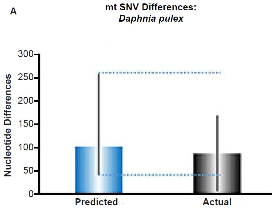
(A) Using the measured SNV mutation rate for the whole mitochondrial DNA (mtDNA) genome in Daphnia pulex, the number of SNV differences was predicted assuming a constant rate of DNA change over 6000 years. This prediction was compared to the maximum SNV difference between Daphnia pulex individuals. The height of each colored bar represented the average (“Predicted” bar) or maximum (“Actual” bar) DNA difference, and the thick black lines represented the 95% confidence interval (“Predicted” bar). As the dotted lines demonstrate, the predicted number of differences captured the maximum current level of mtDNA differences among these individuals. Adapted from Fig. 10 of Jeanson (2015a).
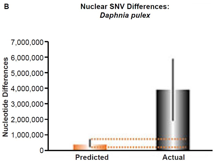
(B) Using the measured SNV mutation rate for the whole nuclear DNA genome in Daphnia pulex, the number of SNV differences was predicted assuming a constant rate of DNA change over 6000 years. This prediction was compared to an estimate of the current levels of nuclear SNV differences among D. pulex individuals. The height of each bar represented the average DNA difference. The thick black lines represented the range of predicted values given the reported error in the mutation rate and given the range of generation time estimates (“Predicted” bar) or the reported range in heterozygosity levels among D. pulex individuals. As the dotted lines demonstrate, predictions clearly underestimated actual differences.
Fig. 5. Contradiction between mtDNA and nuclear DNA SNV clocks in Daphnia pulex.
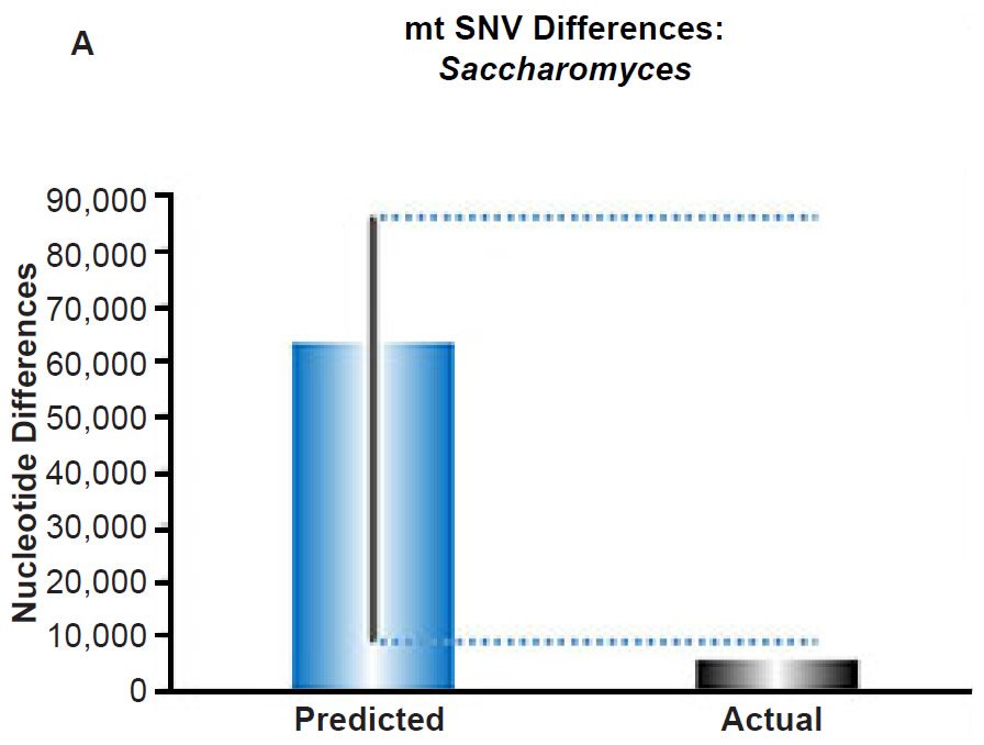
(A) Using the measured SNV mutation rate for the whole mitochondrial DNA (mtDNA) genome in Saccharomyces cerevisiae, the number of SNV differences was predicted assuming a constant rate of DNA change over 6000 years. This prediction was compared to an estimate of the current levels of mtDNA SNV differences between S. cerevisiae and S. paradoxus. The height of each bar represented the average DNA difference, and the thick black lines represented the range of predicted values given the reported error in the mutation rate and given the range of generation time estimates (“Predicted” bar). As the dotted lines demonstrate, the predicted number of differences over-predicted the current level of mtDNA differences between these species.
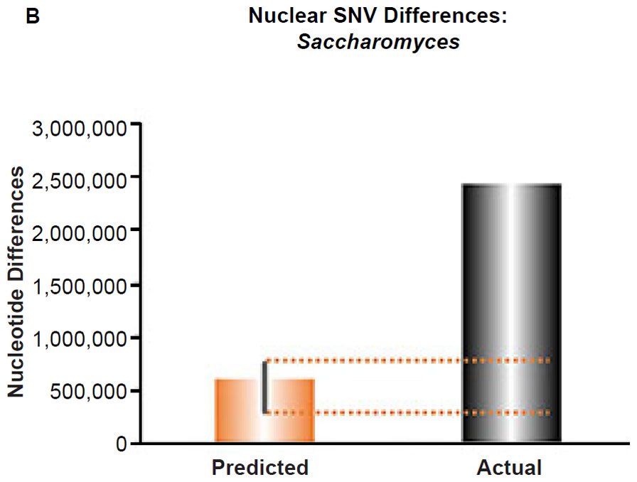
(B) Using the measured SNV mutation rate for the whole nuclear DNA genome in Saccharomyces cerevisiae, the number of SNV differences was predicted assuming a constant rate of DNA change over 6000 years. This prediction was compared to an estimate of the current levels of nuclear SNV differences between S. cerevisiae and S. paradoxus. The height of each bar represented the average DNA difference, and the thick black lines represented the range of predicted values given the reported error in the mutation rate and given the range of generation time estimates (“Predicted” bar). As the dotted lines demonstrate, predictions clearly underestimated actual differences.
Fig. 6. Contradiction between mtDNA and nuclear DNA SNV clocks in yeast.
Since the individuals and species compared in this part of our study represented not only separate phyla but also separate kingdoms, this fact implied that our results were generally true across all ‘kinds.’ Thus, the existence of a whole genome nuclear SNV molecular clock on the YEC timescale was strongly rejected across eukaryotic life.
These conclusions were largely independent of the precise assignment of the ‘kind’ ancestry boundary. Even though our analyses compared species within a single genus or individuals within a single species; and even though previous studies suggested a boundary beyond the level of genus, likely as high as the family level (Wood 2006, 2013), if not higher (Lightner 2010a), special care was exercised to ensure that the individuals or species compared in the mitochondrial SNV analyses were identical to or representative of those in the nuclear SNV analyses. Thus, even if the ‘kind’ ancestry boundary is higher than genus, the main conclusion of this part of the study remained: Mitochondrial and nuclear SNV clocks give conflicting results when members of equivalent taxonomic rank are compared, and explanations for nuclear SNV diversity require invoking different mechanisms than explanations for mtDNA SNV diversity.
(b) The role of mutations
This conclusion did not imply that nuclear SNV mutations have not occurred. From a biblical perspective, mutations have likely been occurring for nearly the entire history of each ‘kind.’ In other words, few YE creationists would deny that the Fall brought instability and imperfection to the “very good” universe that God created; nearly all YE creationists would agree that mutations started at least at the Fall.
Under this model, where mutations do not occur until after the Fall of mankind and after God’s cursing of the creation, the post-Fall time period still represented the vast majority of the natural history of each ‘kind.’ For example, since Adam begot Seth 130 years after Day 6 of the Creation Week (Genesis 5:3), and since Cain and Abel were born after Adam and Eve’s Fall (Genesis 3–4), the Fall itself could not have occurred more than ~127 years after the Creation Week. Furthermore, since Cain and Abel appear to have been at least young men when they had their fatal encounter, the Fall probably occurred shortly after the Creation Week, nearly 6000 years ago (Hardy and Carter 2014). Hence, with a relatively short time span between the Creation Week and the Fall, mutations have been occurring for nearly as long as ‘kinds’ have been in existence.
In addition, mutations are obviously measureable today (e.g., Conrad et al. 2011). The data above (Figs. 3B–6B) clearly demonstrate that 6000 years is sufficient time to generate a small measure (≤25%) of the SNV differences that exist among individuals or species within a ‘kind’ today.
In fact, under the CHNP hypothesis, the SNV mutation rate is theoretically predictable from the assumption of created nuclear SNV diversity in combination with the biblically-appropriate population genetic parameters for each species. For example, in humans, the Scriptural text lays out very clear population genetic constraints. Based on the ages of the patriarchs listed in Genesis 5, human population growth following the Fall was likely dramatic. Adam and Eve lived in a world shortly removed from perfection, and even under today’s conditions, a population size of over 1049 individuals can theoretically be achieved in just 1650 years (Supplemental Table 8). If Adam and Eve were created with nuclear SNV diversity, this massive population growth combined with only 10 generations between Adam and Noah (Genesis 5) entails that most of these created alleles would have been easily passed on to Noah and his family rather than being lost via genetic drift.
Once Noah and his family exited the Ark after the Flood, they and their descendants appear to have undergone rapid population recovery (e.g., Genesis 10), a fact easily explicable with straightforward population modeling (Carter and Hardy 2015). If we ignore the functional impact of any mutations that may have occurred then (i.e., if we assume that new mutations were functionally neutral) and apply standard population genetic assumptions, hardly any new mutations could have been fixed across the entire human population (Carter 2011; Rupe and Sanford 2013).
In addition, shortly after this recovery, intermarriage among the descendants was significantly impeded by the confusion of languages at Babel, an event that was the catalyst for the formation of the major ethnolinguistic groups observable today. As a result, sharing of alleles across major ethnolinguistic groups post-Babel was probably a rare event, and new mutations post-Babel would likely have been unique to each language/ethnic group and, therefore, rare in frequency across the entire human population.
Consistent with these expectations, “rare variants”—nuclear SNV differences defined as those having a minor allele frequency of less than 0.5%—tend to be restricted to single ethnic groups (1000 Genomes Project Consortium et al. 2012). Furthermore, in the 4365 years that have elapsed since the Flood, constant rates of nuclear SNV mutation plausibly explain the origin of these rare variants (Fig. 7). In fact, even the evolutionary community claims to be able to predict the empirically measured human nuclear SNV mutation rate from the rare allele frequency (compare Conrad et al. 2011 to Coventry et al. 2010; then see Nelson et al. 2012).
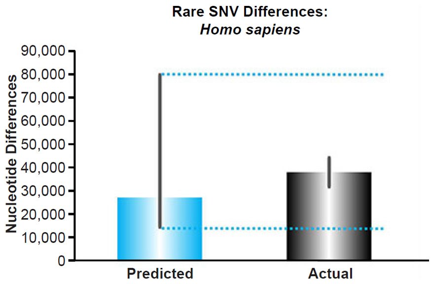
Fig. 7. Mutational origin of rare SNVs in human nuclear DNA. Using the measured SNV mutation rate for the whole nuclear DNA genome in humans, the number of SNV differences was predicted assuming a constant rate of DNA change over 4365 years. This prediction was compared to the current levels of nuclear SNV differences in the category of variants termed “rare variants,” defined as those existing at a frequency of < .5% in the human population. The height of each bar represented the average DNA difference. For the “Predicted” bar, the thick black lines represented the range of predicted values given the reported error in the mutation rate and given the range of generation time estimates. For the “Actual” bar, the thick black lines represented the standard deviation in reported rare variants per individual in extant human non-African populations. As the dotted lines demonstrate, the predicted number of variants overlapped the current range of rare variants.
By contrast, the “common variants”—those nuclear SNV differences that have a minor allele frequency greater than or equal to 5%—tend to be found across various ethnic groups (1000 Genomes Project Consortium et al. 2012). They can be easily explained by fiat creation in Adam and Eve (Carter 2011), implying that their distribution in haplotype blocks around the world would be a function of recombination and gene conversion rates rather than being a product of mutation. As demonstrated above, these common variants are inexplicable by constant rates of nuclear SNV mutation over 6000 years (Fig. 3B), but the assumption of created heterozygosity followed by constant rates of recombination and gene conversion plausibly explains the number of haplotype blocks present in the human population today (Fig. 8).
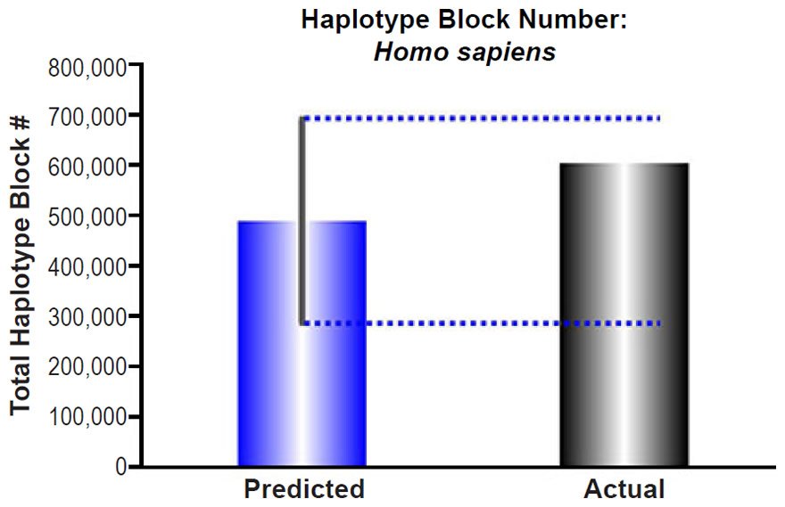
Fig. 8. Created origin of common variants in human nuclear DNA. Assuming that Adam and Eve were created with heterozygosity, the number of haplotype blocks that would result from these created alleles after 6000 years of constant rates of recombination and gene conversion in seven lineages was predicted and compared to an estimate of the current number of haplotype blocks in the human genome. The height of the blue bar represented the average comparative haplotype block number. For the “Predicted” bar, the thick black lines represented the range of predicted values given the reported error in the recombination rate, estimate, and given the range of generation time estimates. As the dotted lines demonstrate, the predicted number of haplotype blocks overlapped the current number.
To clarify, within the world-wide human population, over 84 million total SNV sites have been identified (1000 Genomes Project Consortium et al. 2015). Rare variants, by definition, represent most of these 84 million sites. Since common variants would be present at identical sites in a variety of different individuals, common variants would constitute the minority of sites—they show up frequently but add little to the total number of different sites. By contrast, within each individual, only 3.5–4.3 million SNVs exist on average, and the vast majority of SNVs (>80%) within a single individual are common variants (1000 Genomes Project Consortium et al. 2012, 2015). Thus, within each individual, >80% of the nuclear SNVs (80% by the “common variant” criterion; >98% by Fig. 3B) are due to inheritance of alleles that arose via fiat creation during the Creation Week in Adam and Eve, and a small but significant minority of nuclear SNVs within an individual are due to mutations since Creation.
To underscore the relevance of mutations under the CHNP model, we also found that random SNV mutations to the nuclear DNA sequence appear to be sufficient to explain the origin of some of the allelic diversity today. For example, within a species, mutation can generate far more than the 4–28 alleles that were brought on board the Ark. These new alleles need not be fixed in the entire population so that they define the genotypic differences between species. Instead, they must simply exist in sufficient individuals to be discovered.
A few example calculations demonstrate the ease with which this can occur, and the key to these examples is the definition of an allele. If an allele is defined in terms of a gene unit, then generating “allelic” diversity by mutating just one gene per mutational event produces little diversity. Instead, if an allele is defined as a single genomic position, independent of its relationship to a gene, then enormous allelic diversity can be generated by mutation.
For example, in humans, our current population size of several billion individuals arose from three couples about 4365 years ago (Genesis 9:18–19). To grow the population from eight individuals to several billion, an enormous number of generational events must necessarily occur. At every one of these generational events, new mutations were likely introduced into the population. At current rates, one new mutation occurs per every 100 million base pairs per generation (Conrad et al. 2011) (note the implicit use of the genomic position definition of allele rather than the gene unit definition). If we assume an approximate haploid genome size of 3 billion, this rate equates to about 30 new mutations per haploid generation (1/100,000,000 * 3,000,000,000 = 30).
Under these assumptions, each DNA position has a 1 in 100 million chance of being mutated (3,000,000,000/30 = 100,000,000). Even if our current world-wide population of 7 billion individuals is all that ever was born, the generational events that would have occurred to produce this many individuals would have also resulted in the mutation of each position in our genome 70 times over (7,000,000,000 events/100,000,000 events required per mutation of a particular DNA position = 70 mutations per position). Since there are only four possible DNA nucleotides (A, T, G, C), all of these alleles would be represented somewhere in the population (unless, of course, the allele was lethal). Hence, generating allelic diversity at various genes is straightforward in a few thousand years.
As an aside, allelic diversity need not arise via mutation. Again, if we use the genomic position definition of an allele rather than the gene unit definition, other mechanisms besides mutation can generate allelic diversity. For example, a single gene typically spans thousands of nucleotides, and SNVs might be distributed throughout the gene—for example, at 90 of the nucleotides within the gene. If we allow for the genomic position definition of alleles, every single one of these 90 SNVs may have existed in a heterozygous state in each of the individuals of the pairs brought on board the Ark.
Expanding this single gene example across the entire genome reveals a tremendous potential for allelic diversity on the Ark. In just two diploid individuals, four genome copies exist. Since only four DNA base-pairs exist, virtually every possible genomic position allele (i.e., far more than 4–28 gene unit alleles) could have been present at the time of the Flood, if the individuals were heterozygous.
In summary, constant rates of random mutation over time are able to account for the spectrum of alleles that exist today within a ‘kind’ (see calculations in preceding paragraphs), but constant rates of random mutation are not able to account for the number of SNV differences that are present between species (or individuals) within a ‘kind’ (Figs. 3–6). Therefore, mechanisms other than random mutation are required to justify the current number of SNV differences among species (or individuals) within a ‘kind,’ and the data in Figs. 3–6 suggested created heterozygosity as a plausible hypothesis.
(c) Different mutation rates in different compartments?
The failure of the constant mutation rate hypothesis to explain nuclear SNV diversity implied either that nuclear SNV mutation rates were higher in the past, or that processes other than random mutation generated today’s nuclear SNV diversity. With respect to the former explanation, it is difficult to imagine a process that might accelerate the mutation rate in the nucleus but not in the mitochondria. Neither extracellular nor intracellular processes seem capable of differential mutation acceleration in a manner that would contradict our conclusions.
For example, creationists have postulated that radioactive decay rates were higher in the past (Vardiman, Snelling, and Chaffin 2005). If they were, how would this process affect the nucleus and not the mitochondria? How would alpha particles, ejected electrons, and/or gamma rays (i.e., the products of radioactive decay) selectively target only the nucleus and not the mitochondria? Unless the nucleus somehow possessed currently unknown properties that attracted radioactive particles to itself, it would seem that radioactive decay from extracellular sources would shoot through the cell indiscriminately, affecting both nucleus and mitochondria alike.
Alternatively, unless the nucleus possessed DNA repair machinery that was inferior to the DNA repair machinery in the mitochondria, mutations from extracellular sources would seem to affect both compartments alike. This differential DNA repair hypothesis seems especially unlikely in light of our calculations above (Figs. 3–6). Since current rates of mtDNA SNV mutation are sufficient to account for existing mtDNA SNV diversity (Figs. 3A–6A), it would appear that—under the differential DNA repair hypothesis—every single one of the mtDNA mutations that was produced via accelerated radioactive decay was repaired. This would represent a remarkable biological feat.
Invoking intracellular processes fares no better, especially when examined closely. For example, perhaps DNA repair/maintenance/replication/metabolism in the nucleus uses different enzymes than DNA repair/maintenance/replication/metabolism in the mitochondria. In theory, a mutation to the nuclear DNA enzyme could selectively accelerate nuclear SNV mutation accumulation without affecting mtDNA mutation accumulation—a “mutator allele” hypothesis. At first pass, this explanation might seem plausible.
Upon further reflection, this mechanism faces significant challenges. Presumably, the mutation to the nuclear DNA enzyme would be irreversible, and the effect would continue to this day. Effectively, then, the current nuclear DNA mutation rate would reflect this event. As we already observed, current nuclear SNV mutation rates are insufficient to explain current nuclear DNA diversity (Figs. 3B–6B), which would render this version of the mutator allele hypothesis inadequate.
Alternatively, the mutation to the nuclear DNA enzyme could occur in times past and then, for unknown reasons, be reversed before the present. Aside from being slightly ad hoc, the probability of this type of event is difficult to reconcile with current levels of SNV diversity. As we observed, nuclear SNV diversity exists at only a fraction of the total nuclear DNA positions (Figs. 3B–6B; see also Supplemental Table 6). Since it appears that whole-genome mutational saturation has yet to be reached, invoking a double mutational event at a single position appears improbable, making the mutator allele hypothesis even more unlikely, given current data.
A second potential mechanism for nucleus-selective acceleration of mutation rates follows a similar trajectory. For example, recent studies in Arabidopsis (Yang et al. 2015) indicated that nuclear heterozygosity levels can influence the nuclear SNV mutation rate (Fig. 9). Using the mutation rates analyzed above in Figs. 3B–6B and using published estimates of nuclear DNA heterozygosity from the species that we analyzed, the discoveries in Arabidopsis appeared to be predictive for at least three of the four species that we analyzed above (Fig. 10). Again, at first pass, since nuclear heterozygosity would appear to have no obvious relationship to the mtDNA compartment, these data might suggest that nuclear DNA mutation rates can be accelerated independent of mtDNA mutation rates.
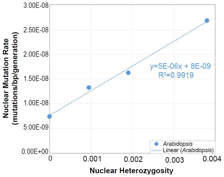
Fig. 9. Nuclear DNA heterozygosity increased nuclear SNV mutation rates in Arabidopsis. The relationship between nuclear DNA heterozygosity and nuclear SNV mutation rates was established previously (Yang et al. 2015), and the raw data from this study used to generate the individual data points. The dotted blue line represented the linear regression function for the four data points, and the blue equation depicted the relationship represented by the line.
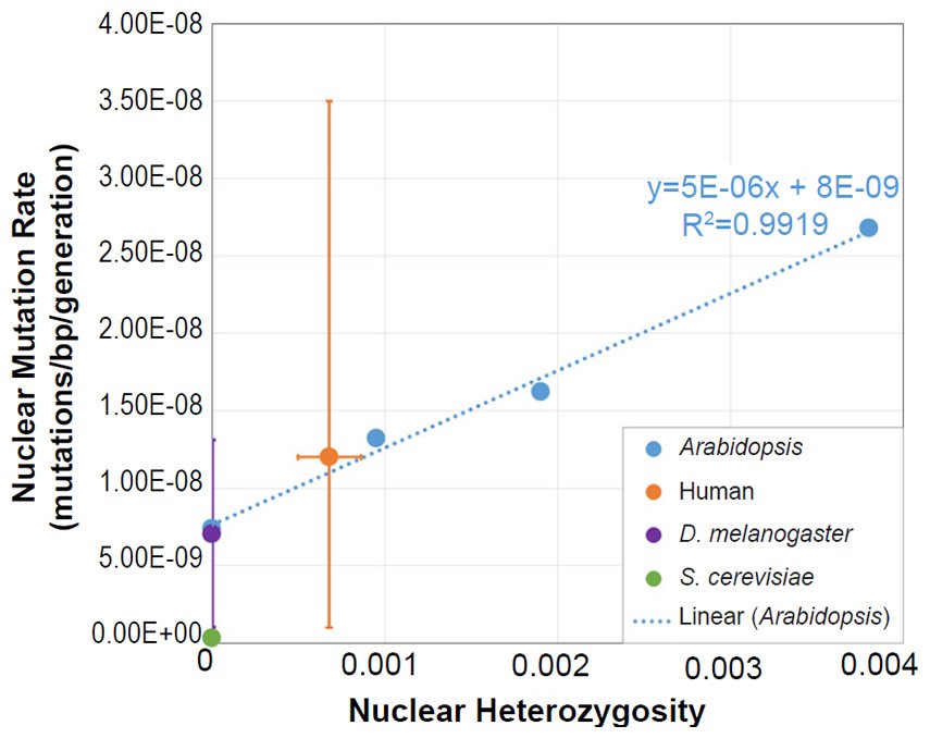
Fig. 10. Relationship between nuclear DNA heterozygosity and nuclear SNV mutation rates in a variety of species. Individual data points from various species were plotted on top of the existing graph in Fig. 9. The dotted blue line represented the linear regression function for the data points from Arabidopsis, and the blue equation depicted the relationship represented by the line. For two of the other species (Humans, D. melanogaster), the linear function derived from the Arabidopsis data nearly predicted the relationship between nuclear DNA heterozygosity and nuclear DNA mutation rates. For the other species (S. cerevisiae), the prediction wasn’t nearly as tight, but the data nonetheless were consistent with relative expectations of lower/zero heterozygosity producing low mutation rates. Colored error bars represented the published ranges or statistical errors associated with the measurements of heterozygosity, of the nuclear SNV mutation rate, or of both for each species.
However, upon more careful inspection, nuclear SNV mutation rates increased only when nuclear heterozygosity levels increased. To refute the CHNP hypothesis, the species with the lowest levels of nuclear DNA heterozygosity should have had the highest levels of mutation rates. Instead, these data show the opposite trend, implying that preexisting heterozygosity was required to generate additional heterozygosity via mutation. In other words, the only way these data from Arabidopsis could have refuted the CHNP model was by assuming the CHNP model at the start—a logical catch-22.
In Daphnia pulex, the nuclear heterozygosity was very high, yet it failed to boost the D. pulex nuclear mutation rate beyond even the most basal level of the Arabidopsis nuclear DNA mutation rate (Fig. 11). Theoretically, it is possible that D. pulex has higher levels of nuclear SNV mutations at lower levels of nuclear SNV heterozygosity. But given the observed relationship in Arabidopsis, and given the apparent relationship in the other species we analyzed (see results above and see on below), this seemed unlikely.
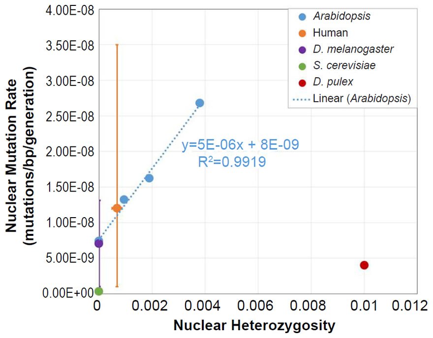
Fig. 11. Relationship between nuclear DNA heterozygosity and nuclear SNV mutation rates in more species. Individual data point from Daphnia was plotted on top of the existing graphs in Figs. 9–10. The dotted blue line represented the linear regression function for the data points from Arabidopsis, and the blue equation depicted the relationship represented by the line. Though the linear function derived from the Arabidopsis data didn’t predict the D. pulex relationship between nuclear DNA heterozygosity and nuclear DNA mutation rates, it did predict the relationship well in other species. Colored error bars represented the published ranges or statistical errors associated with the measurements of heterozygosity, of the nuclear SNV mutation rate, or of both for each species.
Hence, the direction of the relationship between nuclear SNV mutation rates and nuclear SNV heterozygosity supported the central tenets of the CHNP hypothesis.
To be clear, the CHNP model does not reject the possibility of accelerated mutation rates in times past. In fact, under the CHNP hypothesis and in light of the inferences made from the timing of speciation (Jeanson 2015a), the highest historical levels of heterozygosity were likely at Creation or immediately post-Flood, and genetic drift and other processes likely have diluted this concentrated heterozygosity to lower levels (see also sections below on historical changes in SNV levels within ‘kinds’). Consequently, if the heterozygosity-mutation rate relationship discovered in Arabidopsis is generally true across diverse ‘kinds,’ then nuclear mutation rates were likely higher in the past than they are at present.
Even if the Arabidopsis discoveries are unique to plants, the observations made previously—that the comparison of nuclear SNV clocks to mtDNA SNV clocks gives conflicting results when members of equivalent taxonomic rank are compared—still held true, and no mechanisms for accelerating nuclear SNV mutation rates without (1) also accelerating mtDNA SNV mutation rates or (2) adding support to the CHNP hypothesis were obvious. Hence, explanations for mitochondrial SNV diversity still required invoking different mechanisms than explanations for nuclear SNV diversity, and created heterozygosity seemed a very plausible explanation for the latter.
(d) Created heterozygosity in plants
Given the documented relationship between nuclear SNV heterozygosity and nuclear SNV mutation rates in Arabidopsis thaliana (Yang et al. 2015), we explored whether we could make conclusions about our CHNP hypothesis in plants, even in the absence of mtDNA clock data. Using the mutation rate measured in ~homozygous individuals and predicting the amount of mutation accumulation after 6000 years, we found that mutations were insufficient to explain nuclear SNV diversity (Fig. 12).
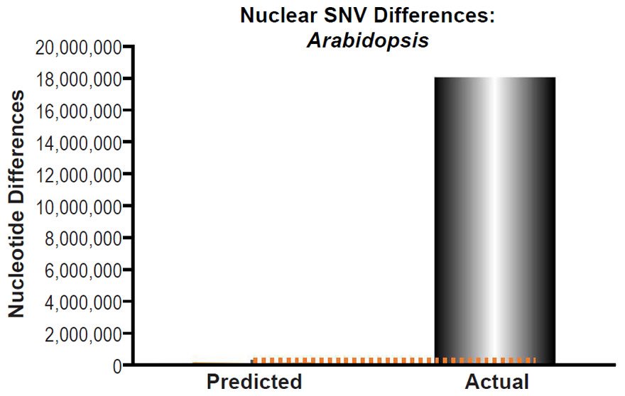
Fig. 12. Inability of mutations to explain Arabidopsis nuclear SNV differences. Using the measured SNV mutation rate for the whole nuclear DNA genome in ~homozygous individuals in Arabidopsis thaliana, the number of DNA differences was predicted assuming a constant rate of DNA change over 6000 years. This prediction was compared to the current levels of nuclear SNV differences between A. thaliana and A. lyrata. The height of each bar represented the average DNA difference, and the thick black lines represented the range of predicted values given the reported error in the mutation rate and given the range of generation time estimates (“Predicted” bar). As the dotted lines demonstrate, predictions clearly underestimated actual differences.
Technically, since mutations would increase the heterozygosity each generation, a strict modeling of the mutation-only hypothesis would require the use of differential equations. However, nearly 6000 years of mutation were required before mutations could have theoretically changed the homozygous state of the species to a heterozygosity value of ~0.001. As Fig. 9 demonstrated, achieving a heterozygosity value of 0.001 would have bumped the mutation rate up by a factor of only ~2. Hence, random mutations over time were insufficient to explain nuclear SNV diversity in 6000 years in Arabidopsis.
Thus, across all three eukaryotic kingdoms—plants, fungi, and animals—random mutations over time were unable to explain genotypic diversity, and created heterozygosity appeared necessary to account for the origin of diverse genotypes across ‘kinds’ in a very broad sampling of life.
(e) Created heterozygosity in other species
We also explored whether nuclear DNA mutation rates were sufficient to explain nuclear SNV diversity in other animal, fungal, and plant species that lacked mtDNA mutation rate data. As with the previous species we analyzed, the relationship between nuclear SNV mutation rates and nuclear heterozygosity in these additional species roughly matched the relationship predicted from the Arabidopsis results (Fig. 13). Specifically, for two species (Pan troglodytes, Mus musculus), the relationship fell very close to the line predicted by Arabidopsis, or, for three species (Heliconius melpomene, Chlamydomonas reinhardtii, Schizosaccharomyces pombe), nuclear heterozygosity was either a product of inbreeding or had already been moved toward a ~homozygous state. The latter condition was especially useful to our purposes since it would eliminate any potential confounding heterozygosity influences on the nuclear SNV mutation rate.
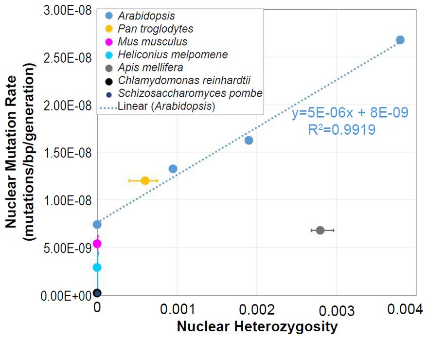
Fig. 13. Relationship between nuclear DNA heterozygosity and nuclear SNV mutation rates in even more species. Individual data points from various species were plotted on top of the existing graph in Fig. 9. The dotted blue line represented the linear regression function for the data points from Arabidopsis, and the blue equation depicted the relationship represented by the line. Though the linear function derived from the Arabidopsis data didn’t predict the Apis mellifera relationship between nuclear DNA heterozygosity and nuclear DNA mutation rates, it approximated the relationship fairly well in the other five species. For three of the species (Pan troglodytes, Mus musculus, and Heliconius melpomene), the linear function derived from the Arabidopsis data nearly predicted the relationship between nuclear DNA heterozygosity and nuclear DNA mutation rates. For the remaining two species (Chlamydomonas reinhardtii, Schizosaccharomyces pombe), the prediction wasn’t nearly as tight, but the data nonetheless were consistent with relative expectations of lower (or zero) heterozygosity producing low mutation rates. Colored error bars represented the published ranges or statistical errors associated with the measurements of heterozygosity, of the nuclear SNV mutation rate, or of both for each species.
Only Apis mellifera fell significantly far away from the predicted line. Nonetheless, a similar relative relationship may hold between nuclear SNV heterozygosity and mutation rate in this species, but on a different absolute scale.
Using the mutation rates from each of these species, we predicted the amount of mutation accumulation after 6000 years. In the animal and plant species, the nuclear SNV predictions severely underestimated existing diversity in the individuals within the species and/or species within the genus (Figs. 14–18).
In contrast, for the fungal species, nuclear SNV predictions overestimated (Fig. 19) SNV diversity within the species. This result may have been due to the fact that SNV diversity was compared within the species rather than between species. For example, when we made fungal nuclear SNV predictions between species instead of individuals within a species (e.g., Fig. 6), the predictions underestimated SNV diversity. Had we compared these latter predictions to SNV diversity within the species, the difference between the prediction and the actual SNV diversity would have disappeared entirely (e.g., compare Saccharomyces predictions in Supplemental Table 6 to SNV diversity among S. cerevisiae individuals in Table S7 of Liti et al. 2009).
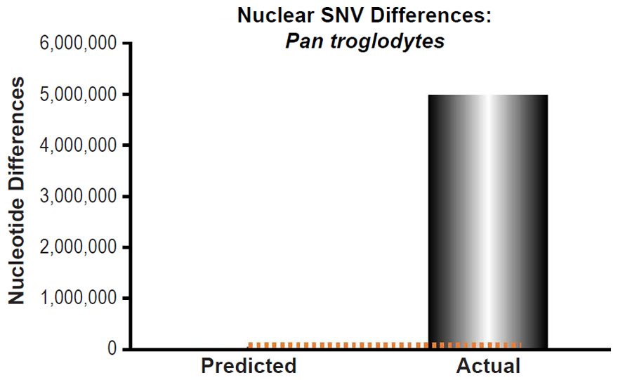
Fig. 14. Inability of mutations to explain chimpanzee nuclear SNV differences. Using the measured SNV mutation rate for the whole nuclear DNA genome in Pan troglodytes, the number of DNA differences was predicted assuming a constant rate of DNA change over 6000 years. This prediction was compared to the highest mean SNV per individual value among the published values for the various Pan troglodytes subspecies. The height of each bar represented the average DNA difference, and the thick black lines represented the range of predicted values given the reported error in the mutation rate and given the range of generation time estimates (“Predicted” bar). As the dotted lines demonstrate, predictions clearly underestimated actual differences.
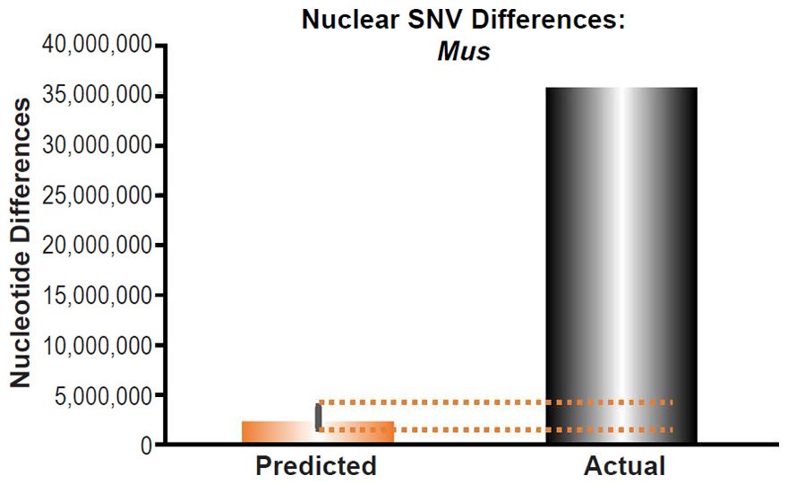
Fig. 15. Inability of mutations to explain mouse nuclear SNV differences. Using the measured SNV mutation rate for the whole nuclear DNA genome in Mus musculus, the number of DNA differences was predicted assuming a constant rate of DNA change over 6000 years. This prediction was compared to the number of SNV differences between laboratory mouse strains and a strain (SPRET/EiJ) derived from Mus spretus. The height of each bar represented the average DNA difference, and the thick black lines represented the range of predicted values given the reported error in the mutation rate and given the range of generation time estimates (“Predicted” bar). As the dotted lines demonstrate, predictions clearly underestimated actual differences.
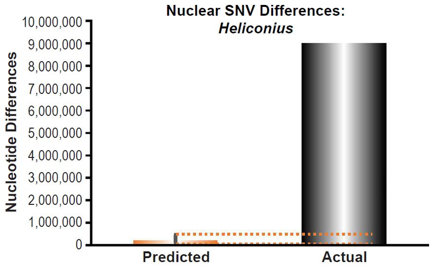
Fig. 16. Inability of mutations to explain butterfly nuclear SNV differences. Using the measured SNV mutation rate for the whole nuclear DNA genome in Heliconius melpomene, the number of DNA differences was predicted assuming a constant rate of DNA change over 6000 years. This prediction was compared to the number of SNV differences between H. melpomene and H. hecale. The height of each bar represented the average DNA difference, and the thick black lines represented the range of predicted values given the reported error in the mutation rate and given the range of generation time estimates (“Predicted” bar). As the dotted lines demonstrate, predictions clearly underestimated actual differences.
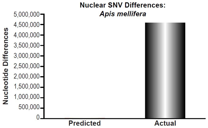
Fig. 17. Inability of mutations to explain honeybee nuclear SNV differences. Using the measured SNV mutation rate for the whole nuclear DNA genome in Apis mellifera, the number of DNA differences was predicted assuming a constant rate of DNA change over 6000 years. This prediction was compared to the highest number of SNVs differences among Apis mellifera subspecies. The height of each bar represented the average DNA difference. As the dotted lines demonstrate, predictions clearly underestimated actual differences.
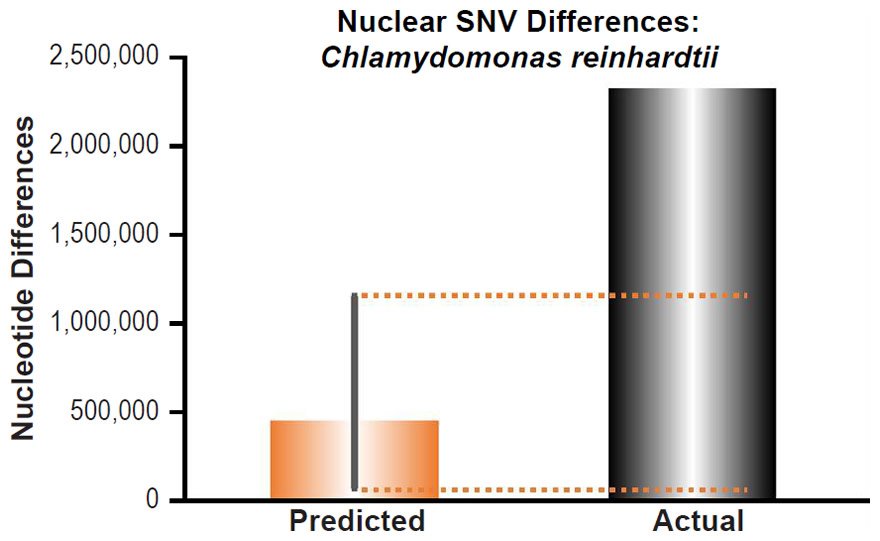
Fig. 18. Inability of mutations to explain Chlamydomonas reinhardtii nuclear SNV differences.Using the measured SNV mutation rate for the whole nuclear DNA genome in Chlamydomonas reinhardtii, the number of DNA differences was predicted assuming a constant rate of DNA change over 6000 years. This prediction was compared to the highest published intra-species SNV difference for C. reinhardtii. The height of each bar represented the average DNA difference, and the thick black lines represented the range of predicted values given the reported error in the mutation rate and given the range of generation time estimates (“Predicted” bar). As the dotted lines demonstrate, predictions underestimated actual differences.
Alternatively, since Schizosaccharomyces pombe is a single-celled organism with a short generation time and a relatively small nuclear genome, mutations might be able to explain a significant amount of nuclear SNV diversity in these types of species. If so, this would be perfectly consistent with the natural processes element of our CHNP model.
Together, these additional mutation rate data added support to our contention that God created a large swath of creatures—at least the animal and plant ones (perhaps, also the fungal ones)—with high amounts of heterozygosity, and that natural processes since the creation event have distributed and added to this pool of SNVs.
(f) The role of non-random mutation
An alternative explanation for some of the nuclear SNV diversity that we observed across diverse species was non-random mutation (non-random with respect to sequence, not base-pair chemistry). For example, in bacteria, non-random mutation appears to occur (Anderson and Purdom 2008). Since bacteria are unicellular and unable to transport themselves long distances, adaptation to changing environments is more difficult, making directed genetic change a plausible answer to the dilemma that each bacterial cell faces.
However, in multicellular eukaryotes (especially mobile ones), it is more difficult to understand how and why a directed mutational mechanism would exist. For permanent genetic change to occur (e.g., the kind of genetic change examined in Figs. 3–6, 14–19), mutations would have to occur in the germline. Since germ cell production is usually internal to each multicellular eukaryote, communicating external needs to internal cells becomes all the more complicated.
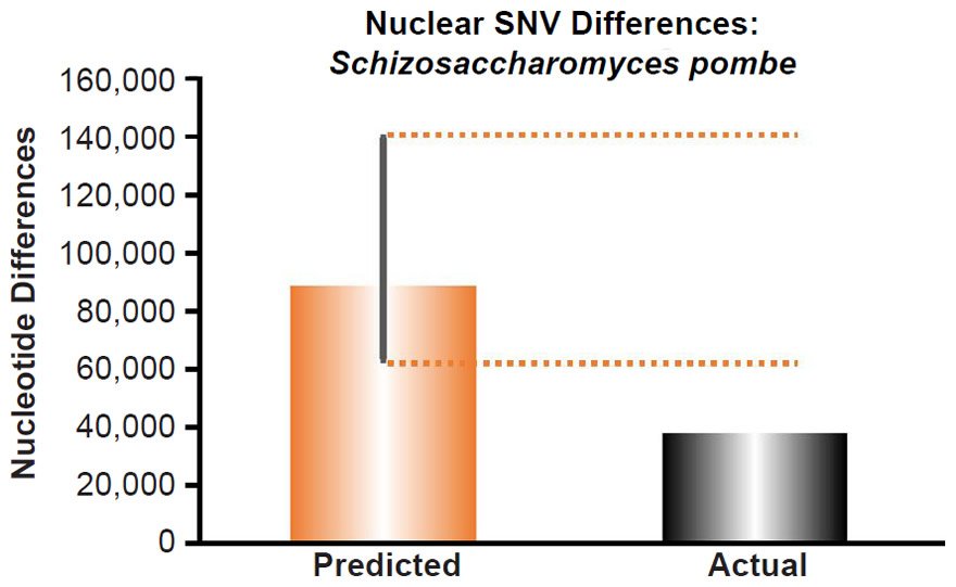
Fig. 19. Mutations explain SNV differences among fission yeast individuals. Using the measured SNV mutation rate for the whole nuclear DNA genome in Schizosaccharomyces pombe, the number of DNA differences was predicted assuming a constant rate of DNA change over 6000 years. This prediction was compared to the average pairwise SNV diversity among S. pombe strains. The height of each bar represented the average DNA difference, and the thick black lines represented the range of predicted values given the reported error in the mutation rate and given the range of generation time estimates (“Predicted” bar). As the dotted lines demonstrate, predictions overestimated actual differences.
Furthermore, though an analogy to directed mutation exists in metazoans, the analogy challenges—rather than helps—the directed mutation model. In the metazoan and human immune systems, a form of directed mutation is used to generate antibody diversity (Chen and Wang 2014). However, the mutations are directed to a very specific subset of the genome and only when triggered by the appropriate stimulus mediated by the complex, genetically-encoded components of the adaptive immune system.
Extrapolating this type of mechanism to the entire genome (where millions of DNA differences exist) would seem to require millions of specific DNA targeting mechanisms and millions of triggers—perhaps millions of genes. In other words, if a single adaptive purpose (e.g., immunity) requires a slew of genetically-encoded biochemical mechanisms, and if a tremendous plethora of adaptive traits exists in the millions of species on the planet today, a non-random explanation for all of this diversity would seem to necessitate a fantastic amount of genetically-encoded biochemical mechanisms dedicated to whole host of adaptive purposes. Specifically, since metazoan genomes typically contain less than 50,000 genes, many of which must encode proteins to fulfill basal functions in the cell such as energy metabolism, cell division and maintenance, etc., the probability of finding a wealth of adaptive biochemical mechanisms in this pool of genes seemed low at present.
Again, for directed mutation to generate permanent genetic change in metazoans, this system would have to alter the germline.
Conversely, for single-celled creatures with small genomes, random mutation over time might be sufficient to explain existing SNV diversity (Fig. 19), obviating the need for non-random mutation.
Hence, until compelling preliminary data can be found to support the non-random hypothesis, it remains just a hypothesis at present.7
Thus, given current data, the created heterozygosity hypothesis in combination with some level of random mutation (e.g., the main genotypic components of the CHNP hypothesis) appeared to be the best explanation for the origin of genotypic SNV diversity in extant ‘kinds.’
(g) Testable predictions
As more and more SNV mutation rates are measured in diverse species, we anticipate that constant rates of nuclear DNA mutation will be found to be insufficient to explain extant genetic diversity. We also expect that nuclear mutation, recombination, and gene conversion rates will be predictable from the relative frequencies of nuclear SNVs among species within a ‘kind,’ as per the precedence in humans. However, since animal, plant, and fungal ‘kinds’ do not have as explicit a record in Scripture as humans do, identifying the “rare” and “common” alleles will be more challenging. Furthermore, unlike humans, animal ‘kinds’ exist as separate species rather than as ethnic groups, and “rare” and “common” variants would need to be defined in terms of species boundaries, not ethnic boundaries.
If, instead, mutation and recombination rates also turn out to be a function of nuclear DNA heterozygosity, as per the precedence in Arabidopsis (Yang et al. 2015), then we predict that the trajectory will mirror the trajectory found for Arabidopsis—preexisting DNA heterozygosity will be required for increasing rates of mutation and recombination/gene conversion.
For those species in which the vast majority of SNVs are inexplicable via constant rates of mutation over time, we predict that these SNVs will turn out to be functional, not non-functional or functionally neutral. In other words, we predict that these SNVs will participate in some way at the molecular level in the biology of each creature in a positive way. Rather than being “junk” DNA, molecular decoration, or harmful to the biology and function of an organism, we expect these variants to contribute to the development, expression, and/or operation of an organism’s traits.
In contrast, we expect most mutationally-derived variants (e.g., a small minority of the SNVs for most of the species and ‘kinds’ we examined) to be functionally neutral or slightly deleterious. Occasionally, some of these mutants might turn out to participate in the speciation process (e.g., see Lang et al. 2012) and therefore be viewed as “beneficial,” but we anticipate that the major effect of these variants will be to impede the normal function of the creature.
Contradictions between any of these predictions and future results would call into question aspects of our CHNP model and would cause us to reevaluate it.
(2) The origin of indels and other nuclear DNA variants
(a) Nuclear indel and SV “clock” analyses
In addition to SNVs, we also examined the origin of other nuclear DNA variants. For example, in the human genome, small insertions and deletions (indels) exist, along with copy number variants (CNVs) [the collective term for larger duplications and deletions], mobile element insertions (MEIs), and inversions (1000 Genomes Project Consortium et al. 2015). While the number of SNVs far exceed the number of all other forms of genetic variation combined, these other variants affect more total base-pairs than SNVs (Sudmant et al. 2015a, 2015b). Theoretically, the non-SNV variation could play a significant role in the speciation process.
To examine the origin of human indel variants, we utilized the fact that the indel and SV (e.g., CNVs, retrotranspositions) mutation rates are known (Kloosterman et al. 2015). Assuming a constant rate of these mutations over 6000 years, we found that our mutation predictions dramatically underestimated the current per-individual indel count by orders of magnitude (Fig. 20; see also data in Supplemental Table 6). In fact, our combined indel + SV mutation rate prediction also dramatically underestimated the current combined CNV and mobile element insertion counts (e.g., median counts per individual; total of 4363 from Table 1 of Sudmant et al 2015b; compare to prediction of 531–1240 in Supplemental Table 6). These results suggested that God created Adam and Eve heterozygous for the vast majority of indels and SVs.
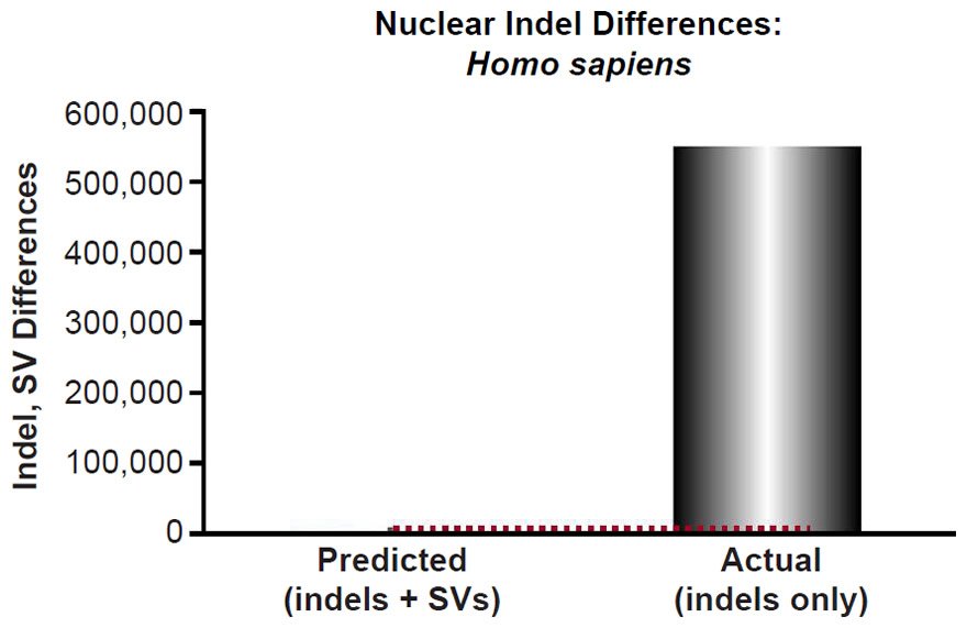
Fig. 20. Created origin of indels and SVs in human nuclear DNA. Using the measured insertion-deletion (indel) and structural variant (SV) mutation rate for the whole nuclear DNA genome in humans, the number of indel differences was predicted assuming a constant rate of DNA change over 6000 years. This prediction was compared to the lowest number of reported indels per individual. The height of each bar represented the average DNA difference. For the “Predicted” bar, the thick black lines represented the range of predicted values given the reported error in the mutation rate and given the range of generation time estimates. As the dotted lines demonstrate, the predicted number of variants severely underestimated the actual number of indel variants, implying that Adam and Eve were created with indel differences within their genomes.
In fact, in light of these results, very little structural variation remained to be explained. Of the SVs characterized by our analyses, inversions and nuclear mitochondrial insertions (NUMTs) were the only categories not yet evaluated. The median number of these per individual is only 37 and 5.3, respectively (Sudmant et al. 2015b). Hence, it appeared that the vast majority of all types of variants carried in each modern human individual stemmed from God’s initial creation of variety in Adam and Eve.
We also explored whether the results in humans were representative of the rest of the species on earth. Unfortunately, no species have genomes as well characterized as the human genome. Nevertheless, we used the available mutation rates and population genetic data to examine whether random mutations over time were sufficient to explain modern indel diversity in three additional species.
When we predicted mutationally-derived indel differences in inbred mice by assuming a constant rate of indel mutations over 6000 years, we found that our mutation predictions dramatically underestimated the current number of indel differences between mouse species by more than an order of magnitude (Fig. 21).
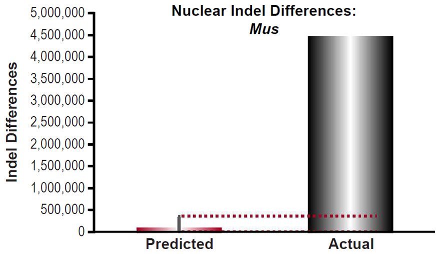
Fig. 21. Created origin of indel variants in mouse nuclear DNA. Using the measured insertion-deletion (indel) mutation rate for the whole nuclear DNA genome in inbred mice, the number of indel differences was predicted assuming a constant rate of DNA change over 6000 years. This prediction was compared to indel divergence between the C57Bl/6 and the SPRET/EiJ mouse strains. The height of each bar represented the average DNA difference. For the “Predicted” bar, the thick black lines represented the range of predicted values given the reported error in the mutation rate and given the range of generation time estimates. As the dotted lines demonstrate, the predicted number of variants severely underestimated the actual number of indel variants, implying that mice individuals were created with indel differences within their genomes.
In Arabidopsis thaliana, the indel mutation rate has been characterized for indels 1 to 3 base-pairs in size (Ossowski et al. 2010). Assuming a constant rate of indel mutations over 6000 years, we found that our mutation predictions dramatically underestimated the current number of 1 to 3 base-pair indel differences between A. thaliana and A. lyrata by more than an order of magnitude (Fig. 22).
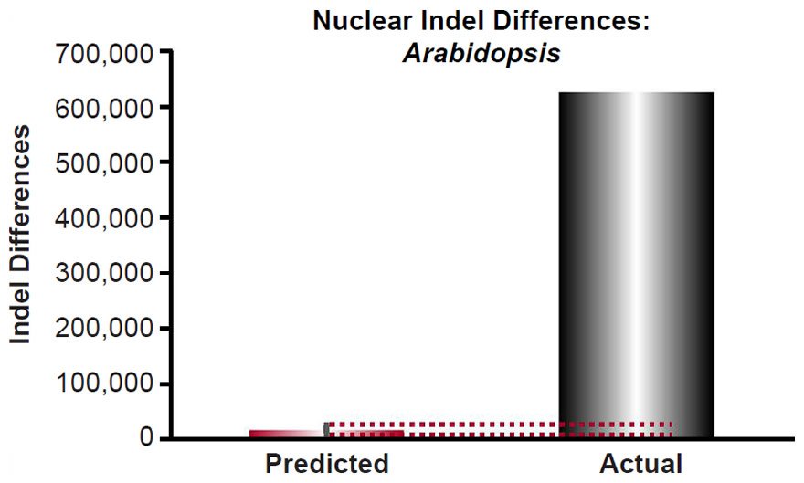
Fig. 22. Created origin of indel variants in Arabidopsis nuclear DNA. Using the measured 1- to 3-base pair insertion-deletion (indel) mutation rate for the whole nuclear DNA genome in Arabidopsis thaliana, the number of 1- to 3-base pair indel differences was predicted assuming a constant rate of DNA change over 6000 years. This prediction was compared to divergence in terms of 1 to 3 base-pair indels between A. thaliana and A. lyrata. The height of each bar represented the average DNA difference. For the “Predicted” bar, the thick black lines represented the range of predicted values given the reported error in the mutation rate and given the range of generation time estimates. As the dotted lines demonstrate, the predicted number of variants severely underestimated the actual number of indel variants, implying that Arabidopsis individuals were created with indel differences within their genomes.
In addition, the recent studies of the relationship between nuclear SNV heterozygosity and nuclear SNV mutation that we discussed above also apply to indels. In A. thaliana individuals, more highly inbred parents (e.g., the Col and Ler lines in Yang et al. 2015) had lower rates of indel mutation than less inbred parents. Presumably, the offspring of the Col and Ler lines (e.g., the F1 offspring which were subsequently crossed, and in which the highest rates of indel mutation were observed) were partially heterozygous for indels as well as for SNVs; therefore, high nuclear heterozygosity positively correlated with higher indel mutation rates (Yang et al. 2015). This implies that the same catch-22 logical loop for the mutational origin of SNVs applies to explanations for the mutational origin of indels—preexisting indels are required to generate more indels via mutation.
A similar relationship might hold in humans as well. A few logical steps between papers suggested as much. In a previous A. thaliana study from 2010 (Ossowski et al.), the measured SNV mutation rate was virtually identical to the SNV rate measured in the inbred parents of the more recent study (Yang et al. 2015). Conversely, humans are more heterozygous than the inbred A. thaliana lines used in the 2015 study, and the human SNV mutation rate is about ~1.6 times higher than the inbred A. thaliana SNV mutation rate (Fig. 10—compare left-most Arabidopsis data point to human data point).
Consistent with this pattern, the A. thaliana mutation rate for 1 to 3 base-pair indels was 4 × 10⁻¹⁰ indels/base-pair/generation (Ossowski et al. 2010) in what was likely an inbred parental line (based on comparison of the SNV rates between the 2010 and 2015 Arabidopsis studies), and the human mutation rate for indels 20 base-pairs or less in length was 6.8 × 10⁻¹⁰ indels/base-pair/generation (Kloosterman et al. 2015), a rate ~1.7 times higher than the A. thaliana rate. Thus, the catch-22 logical loop for the mutational origin of SNVs might apply to indels as well, and it might apply across biological kingdoms.
This logical loop might also exist for mice. In the inbred (e.g., ~homozygous) strain in which the indel mutation rate was measured, the reported rate (1.2 × 10⁻¹⁰ to 6.4 × 10⁻¹⁰ mutations/base-pair/generation) overlapped the reported indel mutation rate (4 × 10⁻¹⁰ indels/base-pair/generation) in inbred Arabidopsis individuals (Ossowski et al. 2010).
Even if a relationship between nuclear indel heterozygosity and nuclear indel mutation rates did not exist in mice, our predictions invoked mutation rates measured in mice that most closely modeled a state without any preexisting (e.g., created) indel heterozygosity—highly inbred (~homozygous) laboratory strains. Hence, mice appeared to have been created heterozygous for indels (Fig. 21) as well as for SNVs (Fig. 15).
In Drosophila, we found that mutations were sufficient to explain some of the interspecies indel diversity. Assuming a constant rate of indel mutations over 6000 years, we found that our mutation predictions overlapped the current number of indel differences between D. melanogaster and D. simulans (Fig. 23).
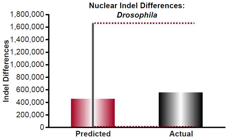
Fig. 23. Mutational origin of indel variants in Drosophila nuclear DNA. Using the measured insertion-deletion (indel) mutation rate for the whole nuclear DNA genome in Drosophila melanogaster, the number of indel differences was predicted assuming a constant rate of DNA change over 6000 years. This prediction was compared to the indel divergence between D. melanogaster and D. simulans. The height of each bar represented the average DNA difference. For the “Predicted” bar, the thick black lines represented the range of predicted values given the reported error in the mutation rate and given the range of generation time estimates. As the dotted lines demonstrate, the predicted number of variants captured the number of indel variants between these species, implying some indel differences were explicable via a constant rate of mutation over time.
However, among the Drosophila species with sequenced genomes, D. simulans is one of the closest relatives to D. melanogaster. When the number of indel differences between D. melanogaster and one of its more distant relatives (e.g., D. pseudoobscura) becomes available, this prediction may become an underestimate and thereby bring the results from all four species into agreement.
Alternatively, as with SNV predictions for Schizosaccharomyces (Fig. 19), organisms with relatively short generation times (e.g., as compared to Arabidopsis and humans) might be able to generate significant genetic diversity via mutation.
Thus, created heterozygosity was necessary to explain the vast majority of genotypic variety present in humans, mice, and in Arabidopsis. Since these results were consistent across two biological kingdoms, we anticipate that they will also turn out to be true in general, even for Drosophila, but mutations might be sufficient to explain genotypic diversity among some species.
Therefore, in eukaryotes, created heterozygosity was necessary for the origin of the vast majority of SNVs and indels, and, since our CHNP model also includes mutations, those variants not explicable by created heterozygosity were still consistent with our CHNP model. Furthermore, in humans, created heterozygosity was necessary for the origin of virtually every class of sequence difference observable today. We expect similar results to hold true for nearly all types of nuclear DNA variants in eukaryotes.
(b) Testable predictions
As more and more indel mutation rates are measured in diverse species, we anticipate that constant rates of nuclear DNA mutation will be found to be insufficient to explain extant genetic diversity.
If mutation and recombination rates also turn out to be a function of nuclear DNA heterozygosity, as per the precedence in Arabidopsis (Yang et al. 2015), then we predict that the trajectory will mirror the trajectory found for Arabidopsis—preexisting DNA heterozygosity will be required for increasing rates of mutation and recombination/gene conversion.
For those species in which the vast majority of indels and SVs are inexplicable via constant rates of mutation over time, we predict that these variants will turn out to be functional, not functionally neutral. In other words, we predict that these indels and SVs will participate in some way at the molecular level in the biology of each creature in a positive way. Rather than being “junk” DNA, molecular decoration, or somehow harmful to the biology and function of an organism, we expect these variants to contribute to the development, expression, and/or operation of an organism’s traits.
In contrast, we expect most mutationally-derived indels and SVs to be functionally neutral or slightly deleterious. Occasionally, some of these mutants might turn out to participate in the speciation process and therefore be viewed as “beneficial,” but we anticipate that the major effect of these variants will be to impede the normal function of the creature.
Contradictions between any of these predictions and future results would call into question aspects of our CHNP model and would cause us to reevaluate it.
(B) Testing the functional relevance of the CHNP model
Ever since Mendel, geneticists have known that simple recombination or reshuffling of a heterozygous nuclear DNA pool can lead to profound phenotypic effects in a single generation. In theory, if ‘kinds’ were front-loaded with enormous heterozygosity, this pool of alleles represented a tremendous source of raw potential for phenotypic diversity. If over 75% of the genomic DNA differences (>90% of the DNA differences for some species and ‘kinds’) present in most metazoan individuals today stemmed from the creation act itself (Figs. 3–6, 14–18, 20–22), then ‘kinds’ have had within themselves the raw material for diversification for nearly as long as they have been in existence.
However, long-standing traditions in molecular biology appeared, at first pass, to put several constraints on this conclusion. Historically, the genome was understood primarily as a factory for producing proteins—hence, the popular “one gene, one protein, one function” moniker. In addition, once the human genome was sequenced, it was observed that the vast majority of sequence did not code for protein, which might suggest that reshuffling of inter-genic DNA variants would have little relevance to the process of speciation. Also, many geneticists were surprised by how few genes the human genome encoded, thereby making it all the more difficult to understand how new combinations of genes could produce such dramatic phenotypic diversity as is present in the world today. Finally, initial gene knockout experiments indicated that only a subset of genes were essential for life, further reducing the pool of genes with potential roles in speciation and adaptation and, consequently, the pool of DNA variants with roles in speciation and adaptation.
Remarkable progress in genetics and molecular biology the last two decades have relieved these constraints and underscored the potential for the reshuffling of millions of DNA differences to functionally play a role in the speciation process. First, an increasing number of proteins appear to be multifunctional (Huberts and van der Klei 2010; Jeffery 2003; Kim and Dang 2005). Testable YEC models suggest that protein multifunctionality exists in mitochondrial proteins (Jeanson 2013), and it may be pervasive across the entire genome—a hypothesis consistent with recent genome-wide gene comparisons across 22 mammal species (Parker et al. 2013). Thus, even if the only functionally-relevant variants were those located in protein coding regions, the potential functional impact of these variants is much greater than first appreciated.
Second, the best studied genome to date, the human genome, has good preliminary evidence for functionality across both the protein-coding and non-coding sections of the genome (ENCODE Project Consortium 2012). Given this precedence as well as recent results from model animals (Gerstein et al. 2010; modENCODE Consortium et al. 2010; Yue et al. 2014), it appears likely that pervasive functionality will be the rule for most animal genomes. If true, this implies that changing the DNA sequence in almost any section of the genome will produce functional—and, perhaps, phenotypic—effects.
In addition, not only the linear order of base-pairs, but also their physical arrangement on (and context within) chromosomes appears to ultimately determine the meaning of a DNA sequence (Wilson et al. 2008). Since non-coding DNA constitutes so much of the genome, this chromosomal context is likely specified by the non-coding DNA, adding further support for a functional role for this genomic compartment.
Third, though the number of genes doesn’t correlate well with organismal complexity (i.e., the relationship seems to plateau), the amount of non-coding DNA shows a striking correlation with organismal complexity (Liu, Mattick, and Taft 2013). Thus, on two counts—correlations and functional studies—non-coding DNA appears to as functionally important as coding DNA, if not more important.
Fourth, experiments in yeast and C. elegans suggest that most, if not all, genes are functional and may even be required for life under the appropriate environmental conditions (Hillenmeyer et al. 2008; Ramani et al. 2012). Again, even if the only functionally-relevant variants were those located in protein coding regions, the potential functional impact of these variants is much greater than first anticipated.
However, while any one of an organism’s DNA variants could potentially play a role in the speciation process, the degree to which each variant impacts function might vary. Genomes appear to be arranged into a hierarchy of modules, with some genes having broader effects than others (Peter and Davidson 2011). Thus, the modular and hierarchical nature of the genome in metazoans implies that altering SNV ratios in the right location may be sufficient to produce an individual with a dramatically new phenotype.
Together, the advances of molecular genetics and developmental biology over the few decades have demonstrated, in theory, the increasing ease with which new species can be formed from a small pool of heterozygous alleles.
Future research will be required to ascertain precisely which variants are necessary and sufficient for species’ phenotypes. The data published thus far are promising, but, for most of the genome, these data still represent preliminary evidence for function.
Nevertheless, in light of the sheer number of DNA differences among species within a ‘kind’ (e.g., millions of SNVs and indels in some of the species; see Figs. 3–6, 12, 14–23), identifying a “single” causative variant in a speciation process is unlikely. As more and more of the genome in each creature appears to be functional, it seems likely that many positions in the genome were involved in speciation events. Hence, if close to 100% of the genome turns out to be functional in each species, the functional relevance of our model will have effectively been demonstrated, and teasing out the individual contributions of each locus will be difficult.
(C) Testing the population genetic plausibility of the CHNP model
(1) Historical changes in DNA variant levels within ‘kinds’’
(a)Historical progression in SNV levels
For the full phenotypic potential of these created alleles in individuals to be realized in a ‘kind’ in the process of speciation, the alleles must be distributed to various populations and subpopulations within ‘kinds.’ To gain a better sense for what types of population genetic processes would need to be involved, we simulated the speciation process at the genetic level.
Under the CHNP model, species within a biological family share a common ancestor, and based on the results above, the vast majority of SNVs in this ancestor were due to the creation act itself. Thus, the highest number of pairwise SNV differences between two species within a biological family provides a minimum estimate of the SNV heterozygosity in the ‘kind’ ancestor.
Comparing nuclear SNV differences between species within a ‘kind’ revealed that, under our model, tremendous SNV heterozygosity would have been present in the ‘kind’ ancestor (Table 6).
Table 6. Historical changes in heterozygosity levels of SNVs across diverse biological families.
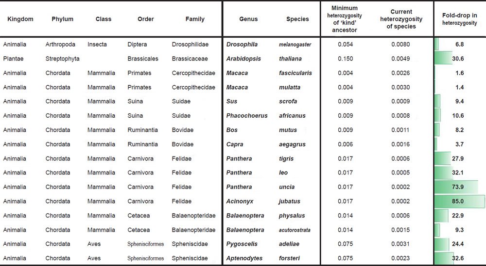
Conversely, comparing SNV differences between individuals within a species revealed that a tremendous reduction in heterozygosity has accompanied the speciation process (Table 6). Across mammal orders, vertebrate classes, and biological kingdoms, all species today possessed fewer heterozygous sites than their ancestors—sometimes an order of magnitude fewer sites (Table 6).
The large range in fold-reduction in heterozygosity values (Table 6) might have been an artifact of the incompleteness of our species representation. Since so few species have a published nuclear DNA sequence, we were forced to compare species over a wide range of ancestry depths. For example, some species recently shared a common ancestor (e.g., the two Macaca species; see the short branch length connecting these two species in Supplemental Fig. 33 in Jeanson 2015a), and, not surprisingly, showed a low value for the reduction in heterozygosity that appeared to accompany the speciation process (Table 6). In contrast, other species shared a common ancestor much further back on the YEC timescale (e.g., the two Balaenoptera species; see the deep branch lengths connecting these two species in Supplemental Fig. 28 in Jeanson 2015a), and, not surprisingly, they showed a much greater drop in heterozygosity (Table 6). Hence, though the fold-drop in heterozygosity varied widely among families, it may have been partly explicable by the species representation levels within the family.
Regardless of the explanation for the variance, the fold-change was always a drop in heterozygosity and never an increase. This observation was consistent with the inferences made from the timing of speciation (Jeanson 2015a). In this previously published analysis, when plotting the time of origin for species within a family via mtDNA comparisons, the rate of speciation appeared to be linear. Though the rate of species formation within a family was constant with time, the number of species within the family increased with time, implying that that speciation rates per species were declining—as if the raw material for speciation was being diluted with time (Jeanson 2015a). The results of the present study (Table 6) are consistent with this inference.
Furthermore, another inference from Jeanson (2015a) was that speciation was still ongoing. Under our CHNP model, since most of the raw genetic material for the speciation process was created during the Creation Week, the potential for speciation would have been present for as long as each ‘kind’ has been in existence—and the potential would continue as long as heterozygosity was still present in extant members of the ‘kind.’ Since heterozygosity still exists in species today (Table 6), our CHNP explains why speciation might still be ongoing.
Finally, the Jeanson (2015a) study demonstrated that the rate of speciation within a family was predictable via a simple formula: The number of extant species divided by the Flood-sensitive timescale (e.g., 4365 years for on-Ark creatures; 6000 years for off-Ark creatures). Another way of stating the same observation is that, once speciation got going for a family, the early results were predictive for the final species numbers in a family. An early start on speciation foretold a good finish. Speciation within a family appeared to be exquisitely sensitive to early post-Flood events.
Our CHNP models offers a plausible explanation as to why. Since heterozygosity levels were highest immediately post-Flood; since heterozygosity represents the raw material for speciation; and since heterozygosity would likely be progressively lost the further and further removed in time that a ‘kind’ found itself, the earlier a ‘kind’ could get the speciation process going, the more likely its descendants would have a larger pool of heterozygous alleles on which to draw for future speciation events. In other words, our CHNP model naturally explains the exquisite sensitivity of ‘kinds’ to the early time points in the speciation process.
To be sure, under our model, once a few loci shift from heterozygous to homozygous during an early post-Creation/post-Flood speciation event, all subsequent shifts need not be towards homozygosity. For example, the initial species that formed in a ‘kind’ post-Flood would have represented shifts from heterozygosity to homozygosity. If the shifts were dramatic, the new species that formed might have been highly homozygous. At a later post-Flood date, a hybridization event between these two very homozygous individuals from these two species might lead to the formation of a new species. [Note the implicit use of a definition of species that is not bound to reproductive isolation.]
Specifically, the hybridization of the two very homozygous parents could result in a highly heterozygous offspring that would then spawn additional offspring, eventually leading to the formation of a new species that itself was more heterozygous than the parental species from which it derived. Hence, under our CHNP model, changes in heterozygosity levels are predicted to result in new species, but the direction of the change need not always be towards more homozygosity.
Thus, whatever population genetic processes might be invoked under our CHNP model, they would need to explain this large reduction in heterozygosity between ‘kind’ ancestors and modern species within each ‘kind.’
(b) Historical progression in indels
As with SNVs, we explored whether indel heterozygosity in ‘kinds’ changed concurrent with the speciation process. Unfortunately, data to perform this analysis existed for only one species—Panthera tigris. Nevertheless, just like the results we obtained for SNVs, we found that, if the felid ancestor was created heterozygous for indels (as our results above would suggest for the vast majority of species, at least those with relatively slow generation times), the process of speciation has resulted in a significant drop in heterozygosity in P. tigris (Table 7).
Table 7. Historical changes in heterozygosity levels of indels in tigers.
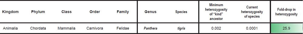
Thus, whatever population genetic processes might be invoked under our CHNP model, they would need to explain this large reduction in heterozygosity in both SNVs and indels between ‘kind’ ancestors and modern species within each ‘kind.’
(c) Population genetic theory
We then explored which population processes were sufficient to account for these changes in heterozygosity with time. Decades of population genetics research have identified the conditions necessary to prevent reductions in heterozygosity in a population—conditions known as Hardy-Weinberg equilibrium (Futuyma 2013; Hamilton 2009). This equilibrium is maintained when a population is infinite in size (e.g., genetic drift must not occur); when input of new alleles via migration of individuals from other populations does not occur; when all the members of the population breed at random; when natural selection doesn’t occur; and when mutation doesn’t occur.
Since the role of mutation appeared to be small in most ‘kinds’ that we examined, we focused on the plausibility of the remaining processes.
(d) Natural selection and linear speciation post-Flood
With respect to natural selection, in the YE community thus far, models have been derived to test the evolutionary mechanism of speciation on the evolutionary timescale (ReMine 2005, 2006; Rupe and Sanford 2013), but few, if any, such calculations have been performed for YEC hypotheses and on YEC timescales.
To fill in this gap, we began by exploring the role that natural selection (defined as preferential survival of individuals to reproduce) might have played in the YEC speciation process. Under the definition just articulated, it naturally follows that the process of natural selection requires sufficient population size to operate.
In other words, defining selection by survival implies that other members of the population die out during a selection event. For this process to be realistic, the surviving individuals must have sufficient numbers to avoid extinction when the next stressor challenges them. For example, if only two individuals survived a stress, this would technically be a natural selection event, but if these two individuals die in a snowstorm the next day or if they fail to reproduce, then the selection event is effectively rendered irrelevant to the speciation process.
To clarify, from a technical perspective, our definition of natural selection largely mirrors the classic definition that Darwin gave:
But if variations useful to any organic being do occur, assuredly individuals thus characterised will have the best chance of being preserved in the struggle for life; and from the strong principle of inheritance they will tend to produce offspring similarly characterised. This principle of preservation, I have called, for the sake of brevity, Natural Selection. (Darwin 1859, 127; italics added)
Since Darwin, natural selection has been defined in numerous ways. To avoid confusion, we exclusively used our definition above.
Before investigating the role of natural selection at the genotypic level in producing specific heterozygosity levels, we first tested the role of natural selection at the phenotypic level in producing recognizable species. Since there are far more DNA differences than species, failure to explain the latter would represent a failure to explain the former, without any need for complex calculations on the millions of DNA differences separating species.
We began by testing whether the post-Flood time period was sufficient to explain speciation via natural selection under the simplest of circumstances. Straightforward population growth calculations in mammals demonstrated that enormous population growth could be achieved in the 4365 years since the Flood (Table 8, which shows only the slowest growing species; see Supplemental Table 8 for full species data and for calculations). Thus, in the few thousand years that have elapsed since the Flood, populations could easily have grown to enormous sizes and then been quickly fractionated by selection into smaller subpopulations of reasonable size to produce new species.
| Family | Genus species | Population size after 4365 years |
|---|---|---|
| … | … | … |
| Delphinidae | Orcinus orca | 1.70E+118 |
| Physeterinidae | Physeter macrocephalus | 9.49E+117 |
| Dugongidae | Dugong dugon | 5.28E+117 |
| Elephantidae | Elephas maximus | 5.17E+116 |
| Elephantidae | Loxodonta africana | 5.17E+116 |
| Delphinidae | Globicephela melas | 6.09E+115 |
| Balaenidae | Balaena mysticetus | 3.02E+96 |
| Delphinidae | Globicephala macrorhynchus | 5.14E+94 |
| Delphinidae | Pseudorca crassidens | 3.96E+65 |
However, this would obviously produce a nonlinear rate of speciation, which appears to contradict the findings of genetics (Jeanson 2015a). Conversely, these population growth conclusions held true in windows of time even smaller than 4365 years—in windows more appropriate to linear speciation rates. As documented previously (Jeanson 2015a; Wood 2011), nearly 75% of all mammal families have 21 species or fewer. At linear (e.g., constant) rates of speciation post-Flood, this would require one speciation event at most once every ~200 years (4365/21 = 208). In 200 years, enormous population growth could still be achieved for most species that we examined. Only a few select off-Ark species could not generate >100,000 individuals in this short timeframe (Table 9, which shows only the slowest growing species; see Supplemental Table 8 for full species data and for calculations). (Note also that the more appropriate timescale for off-Ark ‘kinds’ is 6000 years, not 4365 years.) Hence, if speciation within ‘kinds’ required population growth/reduction cycles every 200 years in order for selection to be responsible for speciation, then natural selection is a generally viable model for this process.
| Family | Genus species | Population size after 200 years |
|---|---|---|
| … | … | … |
| Delphinidae | Stenella attenuata | 5.39E+06 |
| Delphinidae | Orcinus orca | 4.05E+05 |
| Physeteridae | Physeter macrocephalus | 3.95E+05 |
| Dugongidae | Dugong dugon | 3.86E+05 |
| Elephantidae | Elephas maximus | 3.51E+05 |
| Elphantidae | Loxodonta africana | 3.51E+05 |
| Dephinidae | Globicephala melas | 3.21E+05 |
| Delphinidae | Globicephala macrorhynchus | 3.17E+04 |
| Balaenidae | Balaena mysticetus | 2.67E+04 |
| Delphinidae | Pseudorca crassidens | 2.48E+03 |
To investigate more specifically whether population sizes of species within ‘kinds’ could increase on the scale required to produce the extant species diversity seen today, we repeated these models of population growth/reduction with more ‘kind’-appropriate numbers. As described previously, the rate of speciation in extant ‘kinds’ appears to be linear, and it can be predicted from the number of extant species within a family (Jeanson 2015a). Hence, to derive the required rate of speciation within each of the represented ‘kinds,’ we simply divided 4365 years (or 6000 years for Cetaceans and Sirenians) by the number of extant species within each family, and we used this rate to calculate population growth within windows of time appropriate to each family.
These calculations revealed similar trends. The vast majority of the mammal families that we examined could easily reach 100,000 individuals in the window of time specified by the required speciation rate for each family (Table 10). Only 8% of the families had some or all of the species within the family fail to reach 100,000 individuals (Table 10; see Supplemental Table 10 for calculations).
| Families investigated | Families with all species >100,000 individuals | Families with some species <100,000 individuals |
|---|---|---|
| 88 | 81 (92%) | 7 (8%) |
Thus, repeated population growth/reduction cycles were a mathematically plausible option for generating mammal species according to the timelines specified by previously published genetic studies.
The limited taxonomic scope of these calculations implied that further research would be needed before firm conclusions could be made. Today, 151 mammal families exist (Jeanson 2015a), and we sampled only about 60% of them. Within these families, species representation ranged from 100% to less than 1%. Furthermore, we did not model any population growth cycles in birds, reptiles, or amphibians.
Nevertheless, the strong trend of our results suggested that natural selection might be a plausible scenario for at least some of the ‘kinds,’ especially those with few extant species.
Though these cycles assumed survival of the founding pairs for each speciation event, this was a fair assumption. Under a model of a linear rate of speciation, at any point in time only one of the extant populations must spawn a new founder pair. If several populations exist simultaneously, all of them may spawn new founders, and only one of the new pairs has to survive for our calculations to be accurate. Hence, even the survival assumptions of these calculations are not entirely unrealistic.
Thus, even if a selection event required culling most of the existing population within a kind every 50–200 years, the populations of many mammal ‘kinds’ could recover to massive levels very quickly and repeatedly. Hence, at the phenotypic level, selection could have played a significant role in the post-Flood speciation process, at least when measuring selection events according to the timeline of speciation in extant species.
(e) Natural selection and explosive speciation post-Flood
Natural selection may have even played a role in the putative burst of speciation recorded in the Tertiary fossil layers. However, as compared to the linear rates at which extant species formed, the pace with which these Tertiary species formed may have followed a different trajectory. If we assume that the Tertiary period represented ~200 years of time; if we assume that species formed then at a linear rate; and if we divide 200 years by the number of Tertiary species within each family to calculate population growth within windows of time appropriate to each family, only one third of the families that we examined could undergo repeated growth/culling cycles such that each cycle reached a population size of >100,000 individuals (Table 11; see Supplemental Table 11 for calculations).
| Families investigated | Families with all species >100,000 individuals | Families with some species <100,000 individuals |
|---|---|---|
| 82 | 27 (33%) | 7 (67%) |
Instead, if we assume that species formed at an exponential rate during this 200 year window, few temporal instances of sequential founder events would have been required. For example, in the family Camelidae, 126 speciation events happened in Camelidae during the Tertiary time frame (Supplemental Table 3). Under an exponential rate of speciation in which each existing species forms a new species simultaneously, only seven speciation events are required (2x = 126; x = 7).
At exponential rates of speciation, repeated growth/culling cycles were more plausible than at linear rates of speciation. About two-thirds of mammal families that we examined could produce >100,000 individuals in the time frame specified by the number of Tertiary species in the family (Table 12; see Supplemental Table 11 for calculations). This value is higher than the value achieved under the assumption of linear rates of speciation (Table 11), but the percentage is still lower than the value achieved under the assumption of linear rates of speciation in extant families (Table 10).
| Families investigated | Families with all species >100,000 individuals | Families with some species <100,000 individuals |
|---|---|---|
| 82 | 54 (66%) | 28 (34%) |
However, unlike the calculations for linear rates of speciation in extant families, we assumed complete survival of all the founding populations in these calculations for the Tertiary. This is due to the fact that we assumed exponential rates of speciation rather than linear rates. Thus, only if this assumption is true can Tertiary speciation via natural selection be plausible.
Just like the population modeling for extant species, the limited taxonomic scope of the calculations for these Tertiary species implied that further research would be needed before firm conclusions could be made. Nevertheless, the strongly negative trend of our results suggested that natural selection at the phenotypic level would not be a likely scenario for many of the ‘kinds,’ especially those that were highly speciose.
(f) Natural selection of individual DNA variants
In light of the potential for natural selection to play a role on the phenotypic side of the speciation process, we investigated the role of natural selection on the genotypic side of the process. As our historical simulations showed (Tables 6–7), millions of DNA sites have gone from a heterozygous to a homozygous state in the process of speciation.
If selection were to act on individual variants, one-at-a-time, in a sequential manner, then millions of growth-crash cycles would be required. For just 1 million homozygous variants to be selected, a growth-crash cycle would be required once every ~1.6 days (4365 years/1,000,000 selection events * 365.25 days per year = ~1.6 days per selection event). In all the mammal species for which we had data, none of them could produce more than three individuals in this space of time (Supplemental Table 12). Hence, sequential selection of millions of DNA variants was not a plausible scenario by which to reduce heterozygosity on the YEC timescale.
However, these calculations ignore the role of recombination and gene conversion. Because these processes do not swap DNA alleles at every single position in the genome each generation, variants are inherited as linked blocks rather than as independent individual DNA positions. Consequently, selection could potentially operate at the level of linked blocks rather than at the level of individual DNA positions, and it could do so in at least two ways.
First, selection could act on a single DNA variant, and the fact of block inheritance could result in a large swath of alleles being passive “hitch-hikers” along with the selected variant, giving the appearance that many alleles were selected at one time. Over time, due to recombination and gene conversion, the association between the passive alleles and the selected alleles would break down. If too few generations have occurred since the selection event to break down the association, then selection might be able to preserve high levels of homozygosity and, therefore, play a role in the speciation process. However, maintaining this homozygosity permanently would be difficult.
Second, selection could act on the entire block itself. In this case, all of the variants as a single unit might contribute to the selectable phenotype, and the processes of recombination and gene conversion would be working against the selectable phenotype. The size of the block and the rates of recombination and gene conversion would be the key determinants in how quickly and permanently the block could be maintained, if at all.
Together, these results placed significant constraints on the role that natural selection could have played in distributing a heterozygous DNA variant pool to various populations during the speciation process on the YEC timescale. In the future, measurements of the rates of recombination and gene conversion will be critical to testing how much natural selection could have contributed to the reduction of heterozygosity that accompanied the process of speciation within ‘kinds.’
(g) Genetic drift and other population genetic processes
These results did not mean that the CHNP hypothesis was insufficient to explain phenotypic speciation. As mentioned above, natural selection is not the only mechanism by which to alter Hardy-Weinberg equilibrium in a population. Introducing a population substructure via migration or herding can result in effective population sizes that are quite small, and small populations can lose alleles due to genetic drift and inbreeding (Futuyma 2013; Hamilton 2009).
Few, if any, populations today appeared to exist in Hardy-Weinberg equilibrium. No populations are infinite in size, implying that genetic drift is always occurring to some extent. Furthermore, completely random breeding appears to be impossible to maintain, especially in large populations, implying that inbreeding is always occurring to some extent. In short, no realistic populations are in Hardy-Weinberg equilibrium, even if they are not undergoing natural selection. Therefore, if ‘kinds’ were endowed with nuclear DNA diversity from the start, population-level shifts toward homozygosity must have been happening in ‘kinds’ for as long as they have been in existence, implying that population-level phenotypes have been constantly changing, potentially leading to continuous speciation.
To clarify, for new species to form via shifts away from Hardy-Weinberg equilibrium via non-natural-selection population genetic processes, a phenotypic goal or a survival advantage is not necessary. If species are defined by phenotypic traits, then all that is required for the formation of a new species is a new set of traits. For new traits to appear from a pool of individuals who are heterozygous at multiple loci, then all that might be required for new traits to appear is a shift to homozygosity at several of the loci. Hence, so long as shifts towards homozygosity are happening (a.k.a., so long as populations are not in Hardy-Weinberg equilibrium), then new species might be forming.
Furthermore, shifts towards homozygosity can happen extremely rapidly. In just 12 generations of full-sib breeding, heterozygosity can be dropped 10-fold, and in five generations of selfing, heterozygosity drops by a factor of more than 10 (Hamilton 2009). To achieve an 85-fold drop in heterozygosity, less than 30 generations of full-sib breeding are required (Hamilton 2009).
Comparing these calculations to the potential generations elapsed in various ‘kinds’ demonstrated the plausibility of our model. In Table 6, the highest fold-drop in heterozygosity was in felids. Since felid generation times are less than 5 years (Supplemental Table 8), at least 873 felid generations would have passed from the Flood to the present (e.g., 4365 years/5 years per generation = 873 generations). Since heterozygosity could have been lost both via inbreeding and genetic drift, shifts towards homozygosity were more than plausible as a YEC speciation mechanism.
Even some of the slowest reproducing species on record (e.g., Cetaceans; see Table 8) could generate drops in heterozygosity in short order. The highest drop in heterozygosity in Cetaceans was ~23-fold (Table 6), and even in the Cetacean with the slowest generation time (Balaena mysticetus, generation time = 23.6 years; see Supplemental Table 8), 185 generations (e.g., 4365 years/23.6 years per generation = 185 generations) could pass between the Flood and the present. Hence, generating new species from highly heterozygous ancestors via shifts towards homozygosity are not only plausible, they fit the observed data very well.
In summary, since the genotypic results above (Figs. 3–23) argue for the creation of heterozygous individuals (at least in slowly reproducing species) who underwent further mutation after Creation, and since shifts towards homozygosity appear to have been occurring for the entirety of the history of each ‘kind’ (i.e., because maintenance of Hardy-Weinberg equilibrium is nearly impossible in the real world), it is theoretically straightforward to produce a large diversity of species in just a few thousand years via the CHNP model.
Furthermore, in the 4365 years since the Flood and in light of the timing of speciation (Jeanson 2015a) and our simulations above (Tables 6–7), the highest levels of heterozygosity were likely present immediately following the Flood, and genetic drift and other processes likely have diluted this concentrated heterozygosity to lower levels. Consequently, the highest potential for dramatic reshuffling of allelic diversity was immediately following the Flood, implying that the highest potential for phenotypic change and speciation was also in the few years immediately following the Flood. Thus, the CHNP model may also explain the burst of speciation recorded in the Tertiary, if indeed the Flood/post-Flood boundary is located at the K-T.
Together, our data argued that created heterozygosity was necessary to explain the origin of species’ genotypic diversity, and that created heterozygosity in combination with natural process were sufficient to explain species’ phenotypic diversity.
(h) Completing the process of speciation
Under the CHNP model, the final step in the speciation process is the isolation of individuals with homozygous alleles from the rest of the heterozygous population. If isolation does not occur, then homozygous individuals might freely breed with more heterozygous ones, and no permanent genotypic and phenotypic change will occur. Hence, reproductive isolation is necessary for speciation to occur under our model.
Reproductive isolation does not necessitate reproductive incompatibility. Isolation can occur simply via geographic distance. Conversely, many species within families are geographically isolated from one another—e.g., in the family Equidae, the Asian ass species are geographically isolated from the African ass species, and the three species of zebras all occupy fairly distinct regions of Africa.8
This fact underscored the population genetic plausibility of our model. While the mechanisms by which reproductive incompatibility are still a matter of intense investigation, the process of reproductive isolation is straightforward. The habitable surface of the earth is vast, and few families have large numbers of species (Jeanson 2015a), making geographic isolation as a mechanism for reproductive isolation within ‘kinds’ a simple matter.
In the future, additional research will be required to elucidate the mechanism by which reproductive incompatibility occurs. Presumably, the answer to this question will be related to the answer to an equally vexing question, the origin of karyotypic differences (Bedinger 2013) among species within a ‘kind.’ However, both of these puzzles directly impact all explanations for the mechanism of speciation alike, and, therefore, the fact that both puzzles remain research questions did not directly affect the population genetic plausibility of our CHNP model.
(i) Testable predictions and future directions
Shifts away from Hardy-Weinberg equilibrium appear to always be occurring in populations around the globe today and probably have been occurring globally ever since Creation. Hence, the population genetic plausibility of our model is more matter of observational fact and less a question of future predictions.
Conversely, with respect to our model, the major remaining population genetic questions revolve around identifying which of the specific processes—migration, herding, small population sizes, natural selection, mutation, etc.—were responsible for specific speciation events. Realistically, no one specific process was likely at play. Rather, a combination of these processes probably played a role in each speciation event, and separating the relative contributions of each will be a task for future research to solve.
(D) Testing the explanatory scope of the CHNP model
The conclusions we described above on the mechanism by which species originated on the YEC timescale naturally also explain why limits to speciation exist. Under our CHNP model, the vast majority of alleles in most ‘kinds’ arose via direct creation of God during the Creation Week. Consequently, the reshuffling of these alleles (as well as reshuffling of those alleles generated by mutation) within populations is the primary way by which new species arise, according to the CHNP model. Thus, the major fraction of the potential for each ‘kind’ to speciate was hard-wired into each ‘kind’ from the start, implying that changing one ‘kind’ into another would require dramatic genotypic rewiring of a creature. Since upwards of 75% of the genotypic diversity observable today (>90% of the genotypic diversity in some cases) had its origins in the Creation Week, genotypic rewiring does not seem possible apart from a miracle or massive intelligent human intervention. Hence, the CHNP model seemed to simultaneously explain the dramatic but limited speciation with ‘kinds.’
Even in those few examples (e.g., Figs. 19, 23) where intra-’kind’ genotypic differences appear partially derivable via constant rates of mutation over time, we anticipate that sequencing of more species within these ‘kinds’ will eventually bring all results into agreement with the rest of the ‘kinds’ we tested. In other words, we anticipate that created heterozygosity will be required to explain genotypic differences in every ‘kind.’
If this turns out to not be true, the mutation differences that could have accumulated in these ‘kinds’ still represented a small fraction of the total genome size (see Supplemental Table 6). Converting one ‘kind’ into another would likely require mutating significant chunks of the genome into another state. Our mutation rate calculations suggest that 6000 years is not enough time to do so.
Again, as we mentioned in the Introduction to this paper, even if 6000 years was sufficient time to mutate the entire genome within a single lineage within a ‘kind,’ Michael Behe has already elegantly demonstrated that the existence of irreducibly complex structures across various species implies that these structures cannot arise via mutation and natural processes (Behe 1996, 2007). If inter-‘kind’ differences stem from irreducibly complex structures unique to each ‘kind,’ Behe’s observations represent the barrier to inter-‘kind’ conversion.
In summary, we anticipate that the vast majority of metazoan ‘kinds’—perhaps nearly all eukaryotic ‘kinds’—will eventually be shown to derive >90% of their intra-’kind’ genotypic diversity from the creation acts during the Creation Week. If this turns out to be true, then converting one ‘kind’ into another ‘kind’ would appear impossible apart from miraculous genetic intervention. Since Scripture records no such event, our model naturally explains why ‘kinds’ cannot be converted into other ‘kinds.’
(E) The CHNP model versus other hypotheses on the mechanism of speciation
We have shown that our CHNP model is necessary and sufficient for species’ genotypic origins, and is likely also sufficient for species’ phenotypic origins. Our model is genetically plausible, scientifically testable, and comprehensive in explanatory scope. Furthermore, the CHNP model plausibly explains several aspects of the timing of speciation elucidated previously in extant ‘kinds’ (Jeanson 2015a), including the decline in speciation rates per species, the fact of on-going speciation today, and the exquisite sensitivity of final species numbers within a family to early post-Flood speciation events.
With respect to other YEC models, our CHNP model shares some elements with transposon-based models, but only where these models invoke rates of change that are consistent with documented processes today. Our model differs significantly from other models in its strong reliance on created heterozygosity and its use of measureable and plausible rates of mutational change. Furthermore, where other models may have been sought in reaction to the perceived weakness of the original forms of the created heterozygosity model, we believe this reaction is unjustified in light of our current results. In view of these facts, we invite our creationist colleagues to test their own models with the five criteria we outlined above.
While our results represent only a tiny fraction of the diversity of eukaryotic life that exists on our planet, we believe that our results are representative in that they reach across taxonomic ranks even across biological kingdoms. We anticipate that further measurements of mutations rates in various species along with more population genomic data within and between species will serve to strengthen our model and bring into focus the long sought-after answers to the natural history of each species and the mechanism of their origin.
Conclusion
The means by which eukaryotic species’ genotypic and phenotypic diversity arose has been debated for over a century. The comparison between mitochondrial DNA clocks and nuclear DNA clocks reveals the necessity of created heterozygosity in accounting for genotypic diversity within ‘kinds.’ Created heterozygosity in combination with presently observable natural processes (the CHNP model) appears sufficient to explain the vast phenotypic and genotypic diversity observable today, and the CHNP model makes testable predictions by which its strength can be evaluated further in the future. Thus, speciation on the young-earth timescale is not only plausible; it is quickly becoming scientifically superior to any other explanation for the origin of the rich diversity of life on this planet.
Acknowledgments
The initial stages of Nathaniel Jeanson’s research were conducted at the Institute for Creation Research and funded by the Institute for Creation Research. A preliminary draft of this work was presented at the 2014 Creation Research Society meeting, and feedback from the attendees helped refine the conclusions. Special thanks to Georgia Purdom, Roger Patterson, Tommy Mitchell, and Bodie Hodge whose comments on an earlier draft of this manuscript improved it significantly. Also, special thanks to Tim Clarey who alerted Jeanson to the existence of the Paleobiology Database. An extra special thanks to Rob Carter with whom Jeanson has had extensive discussions on population and molecular genetics. This paper would not be possible without the fruit of Rob Carter’s ground-breaking discoveries in the human genome. Also, the librarian at Answers in Genesis, Walt Stumper, has been invaluable in tracking down key papers relevant to this work. Finally, thanks to each of the reviewers whose helpful comments improved an earlier draft of this manuscript.
References
1000 Genomes Project Consortium. 2012. “An Integrated Map of Genetic Variation from 1,092 Human Genomes.” Nature 491 (7422): 56–65.
1000 Genomes Project Consortium. 2015. “A Global Reference for Human Genetic Variation.” Nature 526 (7571): 68–74.
Alroy, J., M. D. Uhen, A. K. Behrensmeyer, A. Turner, C. Jaramillo, P. Mannion, M. T. Carrano, L. W. van den Hoek Ostende, and E. Fara. 2016. “Taxonomic Occurrences of Mammalia Recorded in, Fossilworks, the Evolution of Terrestrial Ecosystems database, and the Paleobiology Database.” Fossilworks. http://fossilworks.org.
Anderson, K. L., and G. Purdom. 2008. A creationist perspective of beneficial mutations in bacteria. In Proceedings of the Sixth International Conference on Creationism. Edited by A. A. Snelling, 73–86. Pittsburgh, Pennsylvania: Creation Science Fellowship and Dallas, Texas: Institute for Creation Research.
Andersson, L. 2013. “Molecular Consequences of Animal Breeding.” Current Opinion in Genetics and Development 23 (3): 295–301.
Austin, S. A., J. R. Baumgardner, D. R Humphreys, A.A. Snelling, L. Vardiman, and K. P. Wise. 1994. “Catastrophic Plate Tectonics: A Global Flood Model of Earth History.” In Proceedings of the Third International Conference on Creationism. Edited by R. E. Walsh, 609–621. Pittsburgh, Pennsylvania: Creation Science Fellowship.
Bedinger, K. 2013. “Chromosome Number Changes Within Terrestrial Mammalian Families.” In Proceedings of the Seventh International Conference on Creationism. Edited by M. Horstemeyer. Pittsburgh, Pennsylvania: Creation Science Fellowship.
Begun, D. J., A. K. Holloway, K. Stevens, L. W. Hillier, Y-P. Poh, M. W. Hahn, P. M. Nista, et al. 2007. “Population Genomics: Whole-Genome Analysis of Polymorphism and Divergence in Drosophila simulans.” PLoS Biology 5 (11): e310.
Behe, M. J. 1996. Darwin’s Black Box. New York, New York: Touchstone.
Behe, M. J. 2007. The Edge of Evolution: The Search for the Limits of Darwinism. New York, New York: Free Press.
Bergman, J., and J. Tomkins. 2012. “Is the Human Genome Nearly Identical to Chimpanzee?—A Reassessment of the Literature.” Journal of Creation 26 (1): 54–60.
Blattner, F. R., G. Plunkett 3rd, C. A. Bloch, N. T. Perna, V. Burland, M. Riley, J. Collado-Vides, et al. 1997. “The Complete Genome Sequence of Escherichia coli K-12.” Science 277 (5331): 1453–1462.
Cao, J., K. Schneeberger, S. Ossowski, T. Günther, S. Bender, J. Fitz, D. Koenig, et al. 2011. “Whole-Genome Sequencing of Multiple Arabidopsis thaliana Populations.” Nature Genetics 43 (10): 956–963.
Carter, R. W. 2011. “The Non-Mythical Adam and Eve! Refuting errors by Francis Collins and BioLogos”. http://creation.com/historical-adam-biologos.
Carter, R., and C. Hardy. 2015. “Modelling Biblical Human Population Growth.” Journal of Creation 29 (1): 72–79.
Cavanaugh, D. P., T. C. Wood, and K. P. Wise. 2003. “Fossil Equidae: A Monobaraminic, Stratomorphic Series.” In Proceedings of the Fifth International Conference on Creationism. Edited by R. L. Ivey, 143–154. Pittsburgh, Pennsylvania: Creation Science Fellowship.
Chen, Z., and J. H. Wang. 2014. “Generation and Repair of AID-initiated DNA Lesions in B Lymphocytes.” Frontiers of Medicine 8 (2): 201–216.
Cho, Y. S., L. Hu, H. Hou, H. Lee, J. Xu, S. Kwon, S. Oh, et al. 2013. “The Tiger Genome and Comparative Analysis with Lion and Snow Leopard Genomes.” Nature Communications 4: 2433.
Conrad, D. F. J. E. M. Keebler, M. A. DePristo, S. J. Lindsay, Y. Zhang, F. Casals, Y. Idaghdour, et al. 2011. “Variation in Genome-Wide Mutation Rates Within and Between Human Families.” Nature Genetics 43 (7): 712–714.
Coventry, A., L. M. Bull-Otterson, X. Liu, A. G. Clark, T. J. Maxwell, J. Crosby, J. E. Hixson, et al. 2010. “Deep Resequencing Reveals Excess Rare Recent Variants Consistent with Explosive Population Growth.” Nature Communications 1: 131.
Daetwyler, H. D., A. Capitan, H. Pausch, P. Stothard, R. van Binsbergen, R. F. Brøndum, X. Liao, et al. 2014. “Whole-Genome Sequencing of 234 Bulls Facilitates Mapping of Monogenic and Complex Traits in Cattle.” Nature Genetics 8: 858–865.
Darwin, C. 1859. On the Origin of Species by Means of Natural Selection, or the Preservation of Favoured Races in the Struggle for Life. London, United Kingdom: John Murray.
Dembski, W. A., and J. Wells. 2008. The Design of Life: Discovering Signs of Intelligence in Biological Systems. Dallas, Texas: The Foundation for Thought and Ethics.
Dong, Y., X. Zhang, M. Xie, B. Arefnezhad, Z. Wang, W. Wang, S. Feng, et al. 2015. “Reference Genome of Wild Goat (Capra Aegagrus) and Sequencing of Goat Breeds Provide Insight into Genic Basis of Goat Domestication.” BMC Genomics 16: 431.
Dobrynin, P., Sh. Liu, G. Tamazian, Z. Xiong, A. A. Yurchenko, K. Krasheninnikova, S. Kliver, et al. 2015. “Genomic Legacy of the African cheetah, Acinonyx jubatus.” Genome Biology 16: 277.
Drosophila 12 Genomes Consortium, A. G. Clark, M. B. Eisen, D. R. Smith, C. M. Bergman, B. Oliver, T. A. Markow. 2007. “Evolution of Genes and Genomes on the Drosophila Phylogeny.” Nature 450 (7167): 203–218.
Druery, C.T., and W. Bateson. 1901. “Experiments in Plant Hybridization.” Journal of the Royal Horticultural Society 26: 1–32.
ENCODE Project Consortium. 2012. “An Integrated Encyclopedia of DNA Elements in the Human Genome.” Nature 489: 57–74.
FAO. 2009. “Status and Trends of Animal Genetic Resources–2008.” Intergovernmental Technical Working Group on Animal Genetic Resources for Food and Agriculture, Fifth Session, Rome, 28–30 January 2009, CGRFA/WG-AnGR-5/09/Inf. 7. ftp://ftp.fao.org/docrep/fao/meeting/016/ak220e.pdf.
Farlow, A., H. Long, S. Arnoux, W. Sung, T. G. Doak, M. Nordborg, and M. Lynch. 2015. “The Spontaneous Mutation Rate in the Fission Yeast Schizosaccharomyces pombe.” Genetics 201 (2): 737–744.
Flowers, J. M., K. M. Hazzouri, G. M. Pham, U. Rosas, T. Bahmani, B. Khraiwesh, D. R. Nelson, et al. 2015. “Whole-Genome Resequencing Reveals Extensive Natural Variation in the Model Green Alga Chlamydomonas reinhardtii.” The Plant Cell 27 (9): 2353–2369.
Franklin, R., and R. G. Gosling. 1953. “Molecular Configuration in Sodium Thymonucleate.” Nature 171 (4356): 740–741.
Futuyma, D. J. 2013. Evolution. Sunderland, Massachusetts: Sinauer Associates, Inc.
Garrigan, D., S. B. Kingan, A. J. Geneva, P. Andolfatto, A. G. Clark, K. R. Thornton, and D. C. Presgraves. 2012. “Genome Sequencing Reveals Complex Speciation in the Drosophila simulans Clade.” Genome Research 22 (8): 1499–1511.
Garrigan, D., S. B. Kingan, A. J. Geneva, J. P. Vedanayagam, and D. C. Presgraves. 2014. “Genome Diversity and Divergence in Drosophila mauritiana: Multiple Signatures of Faster X Evolution.” Genome Biology and Evolution 6 (9): 2444–2458.
Gerstein, M. B., Z. J. Lu, E. L. Van Nostrand, C. Cheng, B. I. Arshinoff, T. Liu, K. Y. Yip, et al. 2010. “Integrative Analysis of the Caenorhabditis elegans Genome by the modENCODE Project.” Science 330 (6012): 1775–1787.
Goffeau, A., B. G. Barrell, H. Bussey, R. W. Davis, B. Dujon, H. Feldmann, F. Galibert, et al. 1996. “Life With 6000 Genes.” Science 274 (5287): 546, 563–567.
Groenen, M.A. M., A. L. Archibald, H. Uenishi, C. K. Tuggle, Y. Takeuchi, M. F. Rothschild, C. Rogel-Gaillard, et al. 2012. “Analyses of Pig Genomes Provide Insight Into Porcine Demography and Evolution.” Nature 491 (7424): 393–398.
Grossniklaus, U., W. G. Kelly, A. C. Ferguson-Smith, M. Pembrey and S. Lindquist 2013. “Transgenerational Epigenetic Inheritance: How Important Is It?” Nature Reviews Genetics 14 (3): 228–235.
Haag-Liautard, C., M. Dorris, X. Maside, S. Macaskill, D. L. Halligan, B. Charlesworth and P. D. Keightley. 2007. “Direct Estimation of Per Nucleotide and Genomic Deleterious Mutation Rates in Drosophila.” Nature 445 (7123): 82–85.
Hamilton, M. B. 2009. Population Genetics. Chichester, United Kingdom: Wiley-Blackwell.
Hardy, C., and R. Carter. 2014. “The Biblical Minimum and Maximum Age of the Earth.” Journal of Creation 28 (2): 89–96.
Harris, E. H. 2001. “Chlamydomonas as a Model Organism.” Annual Review of Plant Physiology and Plant Molecular Biology 52: 363–406.
Heard, E., and R. A. Martienssen. 2014. “Transgenerational Epigenetic Inheritance: Myths and Mechanisms.” Cell 157 (1): 95–109.
Herreid, C. F. II, and S. Kinney. 1967. “Temperature and Development of the Wood Frog, Rana Sylvatica, in Alaska.” Ecology 48 (4): 579–590.
Herskowitz, I. 1998. “Life Cycle of the Budding Yeast Saccharomyces cerevisiae.” Microbiological Reviews 52 (4): 536–553.
Hillenmeyer, M. E., E. Fung, J. Wildenhain, S. E. Pierce, S. Hoon, W. Lee, M. Proctor, et al. 2008. “The Chemical Genomic Portrait of Yeast: Uncovering a Phenotype for all Genes.” Science 320 (5874): 362–365.
Hinch, A. G., A. Tandon, N. Patterson, Y. Song, N. Rohland, C. D. Palmer, G. K. Chen, et al. 2011. “The Landscape of Recombination in African Americans.” Nature 476 (7359): 170–175.
Holt, R. D. 1996. “Evidence for a Late Cainozoic Flood/Post-Flood Boundary.” Creation Ex Nihilo Technical Journal 10 (1): 128–167.
Hu, T. T., P. Pattyn, E. G Bakker, J. Cao, J-F. Cheng, R. M. Clark, N. Fahlgren, et al. 2011. “The Arabidopsis lyrata Genome Sequence and the Basis of Rapid Genome Size Change.” Nature Genetics 43 (5): 476–481.
Huberts, D. H. E. W., and I. J. van der Klei. 2010. “Moonlighting Proteins: An Intriguing Mode of Multitasking.” Biochimica et Biophysica Acta 1803 (4): 520–525.
Jeanson, N. T. 2013. “Recent, Functionally Diverse Origin for Mitochondrial Genes from ~2700 Metazoan Species.” Answers Research Journal 6: 467–501.
Jeanson, N. T. 2015a. “Mitochondrial DNA Clocks Imply Linear Speciation Rates Within ‘Kinds.’” Answers Research Journal 8: 273–304.
Jeanson, N.T. 2015b. “A Young-Earth Creation Human Mitochondrial DNA ‘Clock’: Whole Mitochondrial Genome Mutation Rate Confirms D-loop Results.” Answers Research Journal 8: 375–378.
Jeffares, D. C., C. Rallis, A. Rieux, D. Speed, M. Převorovský, T. Mourier, F. X. Marsellach, et al. 2015. “The Genomic and Phenotypic Diversity of Schizosaccharomyces pombe.” Nature Genetics 47 (3): 235–241.
Jeffery, C. J. 2003. “Moonlighting Proteins: Old Proteins Learning New Tricks.” Trends in Genetics 19 (8): 415–417.
Keane, T. M., L. Goodstadt, P. Danecek, M. A. White, K. Wong, B. Yalcin, A. Heger, et al. 2011. “Mouse Genomic Variation and its Effect on Phenotypes and Gene Regulation.” Nature 477 (7364): 289–294.
Keightley, P. D., R. W. Ness, D. L. Halligan, and P. R. Haddrill. 2014. “Estimation of the Spontaneous Mutation Rate Per Nucleotide Site in a Drosophila melanogaster Full-Sib Family.” Genetics 196 (1): 313–320.
Keightley, P. D., A. Pinharanda, R. W. Ness, F. Simpson, K. K. Dasmahapatra, J. Mallet, J. W. Davey, and C. D. Jiggins. 2015. “Estimation of the Spontaneous Mutation Rate in Heliconius melpomene.” Molecular Biology and Evolution 32 (1): 239–243.
Keith, N., A. E. Tucker, C. E. Jackson, W. Sung, J. I. L. Lledó, D. R. Schrider, S. Schaack, et al. 2016. “High Mutational Rates of Large-Scale Duplication and Deletion in Daphnia pulex.” Genome Research 26 (1): 60–69.
Kellis, M., N. Patterson, M. Endrizzi, B. Birren, and E. S. Lander. 2003. “Sequencing and Comparison of Yeast Species to Identify Genes and Regulatory Elements.” Nature 423 (6937): 241–254.
Kim, J. W., and C. V. Dang. 2005. “Multifaceted Roles of Glycolytic Enzymes.” Trends in Biochemical Sciences 30 (3): 42–50.
Kim, H. L., A. Ratan, G. H. Perry, A. Montenegro, W. Miller, and S. C. Schuster. 2014. “Khoisan Hunter-Gatherers have been the Largest Population Throughout Most of Modern-Human Demographic History.” Nature Communications 5: 5692.
Kloosterman, W. P., L. C. Francioli, F. Hormozdiari, T. Marschall, J. Y. Hehir-Kwa, A. Abdellaoui, E. W. Lameijer, et al. 2015. “Characteristics of De Novo Structural Changes in the Human Genome.” Genome Research 25 (6): 792–801.
Kronforst, M. R. 2008. “Gene Flow Persists Millions of Years after Speciation in Heliconius Butterflies.” BMC Evolutionary Biology 8: 98.
Kronforst, M. R., M. E. B. Hansen, N. G. Crawford, J. R. Gallant, W. Zhang, R. J. Kulathinal, D. D. Kapan, and S. P. Mullen. 2013. “Hybridization Reveals the Evolving Genomic Architecture of Speciation.” Cell Reports 5 (3): 666–677.
Lang, M., S. Murat, A. G. Clark, G. Gouppil, C. Blais, L. M. Matzkin, É. Guittard, et al. 2012. “Mutations in the neverland Gene Turned Drosophila pachea into an Obligate Specialist Species.” Science 337 (6102): 1658–1661.
Langergraber, K. E., K. Prüfer, C. Rowney, C. Boesch, C. Crockford, K. Fawcett, E. Inoue, et al. 2012. “Generation Times in Wild Chimpanzees and Gorillas Suggest Earlier Divergence Times in Great Ape and Human Evolution.” Proceedings of the National Academy of Sciences USA 109 (39): 15716–15721.
Li, C., Y. Zhang, J. Li, L. Kong, H. Hu, H. Pan, L. Xu, et al. 2014. “Two Antarctic Penguin Genomes Reveal Insights into their Evolutionary History and Molecular Changes Related to the Antarctic Environment.” Gigascience 3 (1): 27.
Lightner, J. K. 2008. “Genetics of Coat Color I: The Melanocortin 1 Receptor (MCR1).” Answers Research Journal 1: 109–116.
Lightner, J. K. 2009a. “Genetics of Coat Color II: The Agouti Signaling Protein (ASIP) Gene.” Answers Research Journal 2: 79–84.
Lightner, J. K. 2009b. “Karyotypic and Allelic Diversity Within the Canid Baramin (Canidae).” Journal of Creation 23 (1): 94–98.
Lightner, J. K. 2009c. “Gene Duplications and Nonrandom Mutations in the Family Cercopithecidae: Evidence for Designed Mechanisms Driving Adaptive Genomic Mutations.” Creation Research Society Quarterly 46 (1): 1–5.
Lightner, J. K. 2010a. “Identification of a Large Sparrow-Finch Monobaramin in Perching Birds (Aves: Passeriformes).” Journal of Creation 24 (3): 117–121.
Lightner, J.K. 2010b. “Post-Flood Mutation of the KIT Gene and the Rise of White Coloration Patterns.” Journal of Creation 24 (3): 67–72.
Liti, G., D. M. Carter, A. M. Moses, J. Warringer, L. Parts, S. A. James, R. P. Davey, et al. 2009. “Population Genomics of Domestic and Wild Yeasts.” Nature 458 (7236): 337–341.
Liu, G., J. S. Mattick, and R. J. Taft. 2013. “A Meta-Analysis of the Genomic and Transcriptomic Composition of Complex Life.” Cell Cycle 12 (13): 2061–2072.
Liu, S., E. D. Lorenzen, M. Fumagalli, B. Li, K. Harris, Z. Xiong, L. Zhou, et al. 2014. “Population Genomics Reveal Recent Speciation and Rapid Evolutionary Adaptation in Polar Bears.” Cell 157 (4): 758–794.
Liu, H., X. Zhang, J. Huang, J-Q. Chen, D. Tian, L. D. Hurst, and S. Yang. 2015. “Causes and Consequences of Crossing-Over Evidenced Via a High-Resolution Recombinational Landscape of the Honey Bee.” Genome Biology 16: 15.
Lynch, M., W. Sung, K. Morris, N. Coffey, C. R. Landry, E. B. Dopman, W. J. Dickinson, et al. 2008. “A Genome-Wide View of the Spectrum of Spontaneous Mutations in Yeast.” Proceedings of the National Academy Sciences USA 105 (27): 9272–9277.
Mei, C., H. Wang, W. Zhu, H. Wang, G. Cheng, K. Qu, X. Guang, et al. 2016. “Whole-Genome Sequencing of the Endangered Bovine Species Gayal (Bos frontalis) Provides New Insights into its Genetic Features.” Science Reports 6: 19787.
Miller, J. M., S. S Moore, P. Stothard, X. Liao, and D. W. Coltman. 2015. “Harnessing Cross-Species Alignment to Discover SNPs and Generate a Draft Genome Sequence of a Bighorn Sheep (Ovis canadensis).” BMC Genomics 16: 397.
modENCODE Consortium, S. Roy, J. Ernst, P. V. Kharchenko, P. Kheradpour, N. Negre, M. L. Eaton, et al. 2010. “Identification of Functional Elements and Regulatory Circuits by Drosophila modENCODE.” Science 330 (6012): 1787–1797.
Mora, C., D. P. Tittensor, S. Adl, A. G. B. Simpson, and B. Worm. 2011. “How Many Species are There on Earth and in the Ocean?” PLoS Biology 9 (8): 1–8.
Nelson, M. R., D. Wegmann, M. G. Ehm, D. Kessner, P. St Jean, C. Verzilli, J. Shen, et al. 2012. “An Abundance of Rare Functional Variants in 202 Drug Target Genes Sequenced in 14,002 People.” Science 337 (6090): 100–104.
Ness, R. W., A. D. Morgan, N. Colegrave, and P. D. Keightley. 2012. “Estimate of the Spontaneous Mutation Rate in Chlamydomonas reinhardtii.” Genetics 192 (4): 1447–1454.
Ness, R. W. A. D. Morgan, R. B. Vasanthakrishnan, N. Colegrave, and P. D Keightley. 2015. “Extensive de novo Mutation Rate Variation Between Individuals and Across the Genome of Chlamydomonas reinhardtii.” Genome Research 25 (11): 1739–1749.
Oard, M. J. 1990. An Ice Age Caused by the Genesis flood. El Cajon, California: Institute for Creation Research.
Ochatt, S. J., and R. S. Sangwan. 2008. “In Vitro Shortening of Generation Time in Arabidopsis thaliana.” Plant Cell, Tissue and Organ Culture 93 (2): 133–137.
Ossowski, S., K. Schneeberger, J. I. Lucas-Lledó, N. Warthmann, R. M. Clark, R. G. Shaw, D. Weigel, and M. Lynch. 2010. “The Rate and Molecular Spectrum of Spontaneous Mutations in Arabidopsis thaliana.” Science 327 (5961): 92–94.
Palamara, P. F., L. C. Francioli, P. R. Wilton, G. Genovese, A. Gusev, H. K. Finucane, S. Sankararaman, et al. 2015. “Leveraging Distant Relatedness to Quantify Human Mutation and Gene-Conversion Rates.” American Journal of Human Genetics 97 (6): 775–789.
Pardo-Diaz, C., C. Salazar, S. W. Baxter, C. Merot, W. Figueiredo-Ready, M. Joron, W. O. McMillan, and C. D. Jiggins. 2012. “Adaptive Introgression Across Species Boundaries in Heliconius Butterflies.” PLoS Genetics 8 (6): e1002752.
Parker, G. 1980. “Creation, Mutation, and Variation.” Acts and Facts 9: 11.
Parker, J., G. Tsagkogeorga, J. A. Cotton, Y. Liu, P. Provero, E. Stupka, and S. J. Rossiter. 2013. “Genome-Wide Signatures of Convergent Evolution in Echolocating Mammals.” Nature 502 (7470): 228–231.
Pendragon, B., and N. Winkler. 2011. “The Family of Cats—Delineation of the Feline Basic Type.” Journal of Creation 25 (2): 118–124.
Peter, I. S., and E. H. Davidson. 2011. “Evolution of Gene Regulatory Networks Controlling Body Plan Development.” Cell 144 (6): 970–985.
Pool, J. E., R. B. Corbett-Detig, R. P. Sugino, K. A. Stevens, C. M. Cardeno, M. W. Crepeau, P. Duchen, J. J. Emerson, et al. 2012. “Population Genomics of Sub-Saharan Drosophila melanogaster: African Diversity and Non-African Admixture.” PLoS Genetics 8 (12): e1003080.
Prado-Martinez, J., P. H. Sudmant, J. M. Kidd, H. Li, J. L. Kelley, B. Lorente-Galdos, K. R. Veeramah, A. E. Woerner, et al. 2013. “Great Ape Genetic Diversity and Population History.” Nature 499 (7459): 471–475.
Procházka, E., F. Franko, S. Poláková, and P. Sulo. 2012. “A Complete Sequence of Saccharomyces paradoxus Mitochondrial Genome that Restores the Respiration in S. cerevisiae.” FEMS Yeast Research 12 (7): 819–830.
Ramani, A. K., T. Chuluunbaatar, A. J. Verster, H. Na,V. Vu, N. Pelte, N. Wannissorn, A. Jiao, and A. G. Fraser. 2012. “The Majority of Animal Genes are Required for Wild-Type Fitness.” Cell 148 (4): 792–802.
ReMine, W. J. 2005. “Cost Theory and the Cost of Substitution—A Clarification.” TJ 19 (1): 113–125.
ReMine, W. 2006. “More Precise Calculations of the Cost of Substitution.” Creation Research Society Quarterly 43 (2): 111–120.
Richards, S., Y. Liu, B. R. Bettencourt, P. Hradecky, S. Letovsky, R. Nielsen, K. Thornton, et al. 2005. “Comparative Genome Sequencing of Drosophila pseudoobscura: Chromosomal, Gene, and cis-Element Evolution.” Genome Research 15 (1): 1–18.
Rosenfeld, J. A., C. E. Mason, and T. M. Smith. 2012. “Limitations of the Human Reference Genome for Personalized Genomics.” PLoS One 7(7): e40294.
Rupe, C. L., and J. C. Sanford. 2013. “Using Numerical Simulation to Better Understand Fixation Rates, and Establishment of a New Principle: Haldane’s Ratchet.” In Proceedings of the Seventh International Conference on Creationism. Edited by M. Horstemeyer. Pittsburgh, Pennsylvania: Creation Science Fellowship.
Schrider, D. R., D. Houle, M. Lynch, and M. W. Hahn. 2013. “Rates and Genomic Consequences of Spontaneous Mutational Events in Drosophila melanogaster.” Genetics 194 (4): 937–954.
Shan, E. L. 2009. “Transposon Amplification in Rapid Intrabaraminic Diversification.” Journal of Creation 23 (2): 110–117.
Sudmant, P. H., S. Mallick, B. J. Nelson, F. Hormozdiari, N. Krumm, J. Huddleston, B. P. Coe, et al. 2015a. “Global Diversity, Population Stratification, and Selection of Human Copy-Number Variation.” Science 349 (6253): DOI: 10.1126/science.aab3761.
Sudmant, P. H., T. Rausch, E. J. Gardner, R. E. Handsaker, A. Abyzov, J. Huddleston, Y. Zhang, et al. 2015b. “An Integrated Map of Structural Variation in 2,504 Human Genomes.” Nature 526 (7571): 75–81.
Terborg, P. 2008. “Evidence for the Design of Life: Part 2—Baranomes.” Journal of Creation 22 (3): 68–76.
Terborg, P. 2009. “The Design of Life: Part 3—An Introduction to Variation-Inducing Genetic Elements.” Journal of Creation 23 (1): 99–106.
Tomkins, J. P. 2011. “Genome-Wide DNA Alignment Similarity (Identity) for 40,000 Chimpanzee DNA Sequences Queried against the Human Genome is 86–89%.” Answers Research Journal 4: 233–241.
Tomkins, J. P. 2013a. “Comprehensive Analysis of Chimpanzee and Human Chromosomes Reveals Average DNA Similarity of 70%.” Answers Research Journal 6: 63–69.
Tomkins, J. P. 2013b. “The Human Beta-Globin Pseudogene is Non-Variable and Functional.” Answers Research Journal 6: 293–301.
Tomkins, J. P. 2013c. “Alleged Human Chromosome 2 ‘Fusion Site’ Encodes an Active DNA Binding Domain Inside a Complex and Highly Expressed Gene—Negating Fusion.” Answers Research Journal 6: 367–375.
Tomkins, J. P. 2014. “Comparison of the Transcribed Intergenic Regions of the Human Genome to Chimpanzee.” Creation Research Society Quarterly 50 (4): 212–221.
Tomkins, J., and J. Bergman. 2012. “Genomic Monkey Business—Estimates of Nearly Identical Human-Chimp DNA Similarity Re-evaluated Using Omitted Data.” Journal of Creation 26 (1): 94–100.
Tomkins, J. P., and J. Bergman. 2015. “Evolutionary Molecular Genetic Clocks—A Perpetual Exercise in Futility and Failure.” Journal of Creation 29 (2): 26–35.
Tucker, A. E., M. S. Ackerman, B. D. Eads, S. Xu, and M. Lynch. 2013. “Population-Genomic Insights into the Evolutionary Origin and Fate of Obligately Asexual Daphnia pulex.” Proceedings of the National Academy of Sciences USA 110 (39): 15740–15745.
Uchimura, A., M. Higuchi, Y. Minakuchi, M. Ohno, A. Toyoda, A. Fujiyama, I. Miura, S. Wakana, J. Nishino, and T. Yagi. 2015. “Germline Mutation Rates and the Long-Term Phenotypic Effects of Mutation Accumulation in Wild-Type Laboratory Mice and Mutator Mice.” Genome Research 25 (8): 1125–1134.
Vardiman, L., A. A. Snelling, and E. F. Chaffin, eds. 2005. Radioisotopes and the Age of the Earth: Results of a Young-Earth Research Initiative. Vol. 2. El Cajon, California: Institute for Creation Research and Chino Valley, Arizona: Creation Research Society.
Venn, O., I. Turner, I. Mathieson, N. de Groot, R. Bontrop, and G. McVean. 2014. “Strong Male Bias Drives Germline Mutation in Chimpanzees.” Science 344 (6189): 1272–1275.
Wallberg, A., F. Han, G. Wellhagen, B. Dahle, M. Kawata, N. Haddad, Z. L. P. Simões, et al. 2014. “A Worldwide Survey of Genome Sequence Variation Provides Insight Into the Evolutionary History of the Honeybee Apis mellifera. Nature Genetics 46 (10): 1081–1088.
Wang, J., H. C. Fan, B. Behr, and S. R. Quake. 2012. “Genome-wide Single-Cell Analysis of Recombination Activity and De Novo Mutation Rates in Human Sperm.” Cell 150 (2): 402–412.
Wang, K., Q. Hu, H. Ma, L. Wang, Y. Yang, W. Luo, and Q. Qiu. 2014. “Genome-wide Variation Within and Between Wild and Domestic Yak.” Molecular Ecology Resources 14 (4): 794–801.
Watson, J. D., and F. H. Crick. 1953. “Molecular Structure of Nucleic Acids: A Structure for Deoxyribose Nucleic Acid.” Nature 171 (4356): 737–738.
Williams, A. L., G. Genovese, T. Dyer, N. Altemose, K. Truax, G. Jun, N. Patterson, et al. 2015. “Non-crossover Gene Conversions Show Strong GC Bias and Unexpected Clustering in Humans.” Elife 4: :e04637.
Whitmore, J. H., and P. Garner. 2008. “Using Suites of Criteria to Recognize Pre-Flood, Flood, and Post-Flood Strata in the Rock Record with Application to Wyoming (USA). In Proceedings of the Sixth International Conference on Creationism. Edited by A. A. Snelling, 425–448. Pittsburgh, Pennsylvania: Creation Science Fellowship and Dallas, Texas: Institute for Creation Research.
Whitmore, J. H., and K. P. Wise. 2008. “Rapid and Early Post-Flood Mammalian Diversification Evidenced in the Green River Formation.” In Proceedings of the Sixth International Conference on Creationism. Edited by A. A. Snelling, 449–457. Pittsburgh, Pennsylvania: Creation Science Fellowship and Dallas, Texas: Institute for Creation Research.
Wilkins, M. H. F., A. R. Stokes, and H. R. Wilson. 1953. “Molecular Structure of Nucleic Acids: Molecular Structure of Deoxypentose Nucleic Acids.” Nature 171 (4356): 738–740.
Wilson, M. D., N. L. Barbosa-Morais, D. Schmidt, C. M. Conboy, L. Vanes, V. L. Tybulewicz, E. M. Fisher, S. Tavaré, and D. T. Odom. 2008. “Species-Specific Transcription in Mice Carrying Human Chromosome 21.” Science 322 (5900): 434–438.
Wise, K. P. 2005. “The Flores Skeleton and Human Baraminology.” Occasional Papers of the BSG 6: 1–13.
Wood T. C. 2002. “The AGEing Process: Rapid Post-Flood, Intrabaraminic Diversification Caused by Altruistic Genetic Elements (AGEs).” Origins (GRI) 54: 5–34.
Wood, T. C. 2003a. “Perspectives on AGEing, a Young-Earth Creation Diversification Model.” In Proceedings of the Fifth International Conference on Creationism. Edited by R. L. Ivey, 479–489. Pittsburgh, Pennsylvania: Creation Science Fellowship.
Wood, T. C. 2003b. “Mediated Design.” Acts and Facts 32 (9).
Wood, T. C. 2006. “The Current Status of Baraminology.” Creation Research Society Quarterly 43 (3): 149–158.
Wood, T. C. 2011. “Terrestrial Mammal Families and Creationist Perspectives on Speciation.” Journal of Creation Theology and Science Series B: Life Sciences 1: 2–5.
Wood, T. C. 2013. “A Review of the Last Decade of Creation Biology Research on Natural History, 2003–2012.” In Proceedings of the Seventh International Conference on Creationism. Edited by M. Horstemeyer. Pittsburgh, Pennsylvania: Creation Science Fellowship.
Wood, T. C., and D. P. Cavanaugh. 2001. “A Baraminological Analysis of Subtribe Flaveriinae (Asteraceae: Helenieae) and the Origin of Biological Complexity.” Origins 52: 7–27.
Yan, G., G. Zhang, X. Fang, Y. Zhang, C. Li, F. Ling, D. N. Cooper, et al. 2011. “Genome Sequencing and Comparison of Two Nonhuman Primate Animal Models, the Cynomolgus and Chinese Rhesus Macaques.” Nature Biotechnology 29 (11): 1019–1023.
Yang, S., L. Wang, J. Huang, X. Zhang, Y. Yuan, J-Q. Chen, L. D. Hurst, and D. Tian. 2015. “Parent-Progeny Sequencing Indicates Higher Mutation Rates in Heterozygotes.” Nature 523 (7561): 463–467.
Yim, H-S., Y. S. Cho, X. Guang, S. G. Kang, J-Y. Jeong, S-S. Cha, H-M. Oh, et al. 2014. “Minke Whale Genome and Aquatic Adaptation in Cetaceans.” Nature Genetics 46 (1): 88–92.
Yue, F., Y. Cheng, A. Breschi, J. Vierstra, W. Wu, T. Ryba, R. Sandstrom, et al. 2014. “A Comparative Encyclopedia of DNA Elements in the Mouse Genome.” Nature 515 (7527): 355–364.
Zhu, Y. O., M. L. Siegal, D. W. Hall, and D. A. Petrov. 2014. “Precise Estimates of Mutation Rate and Spectrum in Yeast.” Proceedings of the National Academy of Sciences USA 111 (22): E2310–2318.
Supplemental Files
Supplemental Table 1. Timeline of GenBank growth.
Supplemental Table 2. Calculation of total species and family numbers in vertebrates other than fish.
Supplemental Table 3. Analysis of fossil mammal data from the Paleobiology Database.
Supplemental Table 4. Raw calculations for tabulation of breed numbers.
Supplemental Table 5. Raw pairwise mtDNA comparison data for Daphnia pulex individuals.
Supplemental Table 6. Raw calculations for molecular clock predictions and comparisons.
Supplemental Table 7. Raw numbers for plotting heterozygosity-mutation rate relationship.
Supplemental Table 8. Raw calculations for population growth predictions from AnAgeing Database.
Supplemental Table 9. Common names for taxonomic designations used in this study.
Supplemental Table 10. Raw calculations for population growth predictions from AnAgeing Database using extant-appropriate, family-specific time intervals.
Supplemental Table 11. Raw calculations for population growth predictions from AnAgeing Database using Tertiary-appropriate, family-specific time intervals.
Supplemental Table 12. Raw calculations for population growth predictions from AnAgeing Database using constraints imposed by intra-‘kind’ DNA differences.


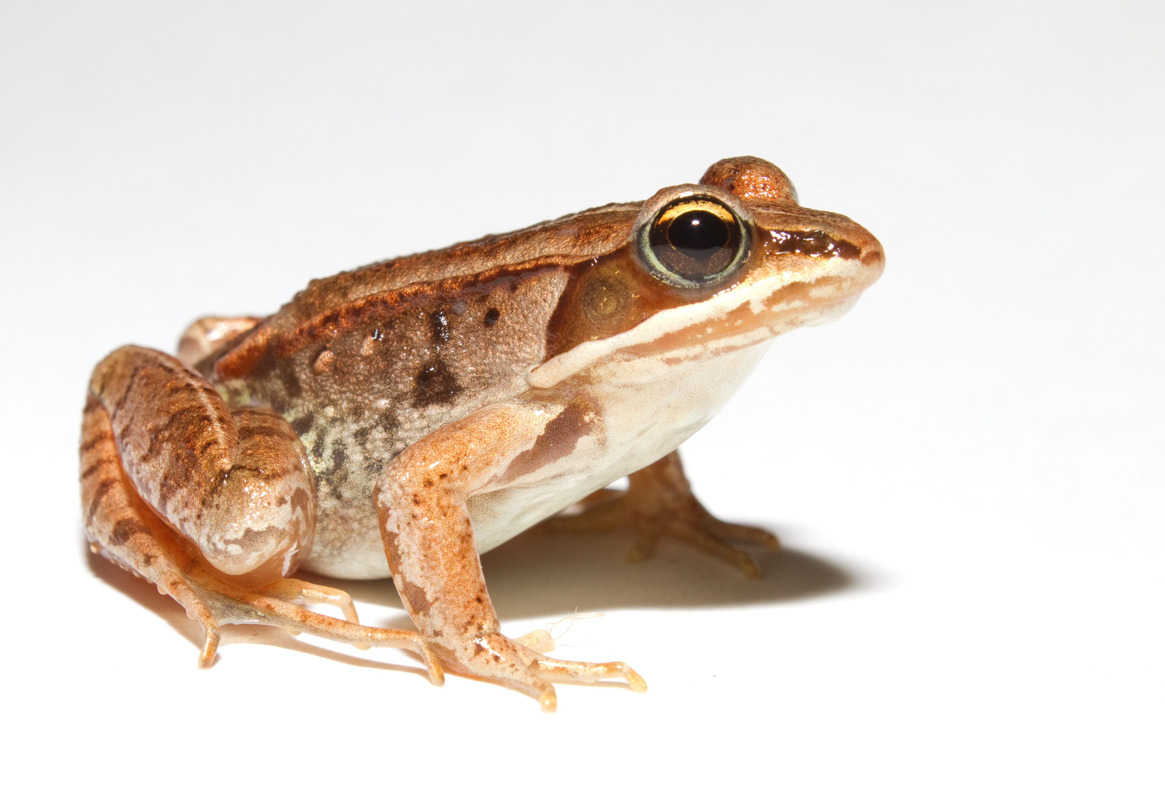