New Method to Assess the Luminosity Function of Galaxies

Introduction

Recent data from the Sloan Digital Sky Survey (SDSS)1 have revealed large-scale patterns in the distribution of galaxies in the local universe. Some patterns appear to be galacto-centric, as if galaxies were organized into large concentric spheres centered roughly on our local group of galaxies: the “bulls-eye effect.” If galaxies are truly organized in such a way, this would strongly challenge the standard secular model of universal origins which presupposes that our position in space is not privileged. However, there are several different ways in which the bulls-eye effect might appear in SDSS maps even if galaxies are not actually organized in such a way. The apparent patterns could be due to a selection effect: an artifact in data analysis arising from the way in which the data were collected. It is essential that we have a proper understanding of biases in SDSS data before we can make any substantial claim about quantized redshifts. This paper discusses how to understand and ameliorate biases due to instrumentation that could produce galacto-centric artifacts. The results will allow other astronomers to more accurately assess SDSS data.

As one example, a map of galaxy positions might show increased galaxy density at certain positions, not because there are genuinely more galaxies at such positions, but because galaxies are easier to detect at those positions for whatever reason. After all, the SDSS is not capable of detecting all galaxies. Some are too faint. Others are lost in the glare of an interloping bright star, and so on. Hypothetically, if galaxies were easier to detect at certain redshifts, then the resulting maps will show concentric spheres (around any hypothetical observer regardless of location) even though the true distribution of galaxies may be completely uniform. For this reason, we must determine the selection function: the fraction of galaxies detected in SDSS compared to the true number of galaxies at a given location. When we divide our observed galaxy density at a given distance by the selection function, the result is (by definition) the true galaxy density at such a distance.

The SDSS is a magnitude-limited survey, meaning that it detects essentially all galaxies that are brighter than a particular instrumentally-imposed threshold.2 In assessing the distribution of galaxies in a magnitude-limited survey, one must deal with the Malmquist bias—the fact that intrinsically faint galaxies can be detected nearby but not at large distance. The Malmquist bias results in surveys that are biased toward bright objects simply because bright objects are easier to detect. The Malmquist bias also results in surveys in which galaxy density seems to fall off with increasing distance simply because galaxies appear fainter and are consequently harder to detect with increasing distance. Only the very brightest galaxies can be detected at the farthest distances in the survey.

Since the apparent brightness of any light emitter falls off as 1/r² (where r is the distance3 to the observer) we might naïvely expect that the Malmquist bias would result in maps in which galaxy density falls off smoothly with increasing distance, and therefore could not possibly be responsible for concentric spheres of enhanced galaxy number density in the resulting maps. That is, we might expect any artifacts introduced by the Malmquist bias to be smooth and non-periodic (in redshift). However, this is not necessarily so. Suppose for example that galaxies exist in preferred brightnesses, such that a histogram of galaxy brightnesses shows periodic local maxima. As one hypothetical scenario, imagine that galaxies with even absolute magnitudes outnumber galaxies with odd absolute magnitudes, so the histogram of brightnesses shows a wave pattern. In this case, the resulting uncalibrated map of galaxy positions will show apparent enhancements in galaxy density as a function of distance—concentric spheres of enhanced density. This is because each peak in the brightness histogram will correspond to a particular maximum distance at which galaxies of that brightness can be detected:

Suppose, for example, that the number of galaxies drops sharply at luminosities higher than L—some arbitrary reference luminosity. Then at distances beyond the maximum distance at which L can be detected, we would not detect very many galaxies since only the few galaxies brighter than L can be seen. Hence, an irregular or unexpected distribution of galaxy brightness will result in apparent geocentric shells of enhanced or depleted density at certain distances from earth—unless such biases are understood and removed.

Therefore, if we are to distinguish real features in SDSS galaxy plots from artifacts, we must compute (1) the luminosity function and (2) the selection function. The luminosity function [Φ(M)] is basically a histogram of galaxy brightnesses. More precisely, Φ(M)dM is the fraction of galaxies that exist between two brightness values, or absolute magnitudes4: [M, M + dM]. The selection function (S) is the number of galaxies detected at a given distance/redshift divided by the true number of galaxies at that same distance/redshift.5 Since light falls off as 1/r², the selection function can be estimated from the luminosity function and the limiting magnitude of the detection instrument, as will be shown. Only if the selection function is smooth can we conclude that peaks in redshift space are real rather than artifacts.

Traditional Methods

Since brighter galaxies are easier to detect, they are oversampled in magnitude-limited surveys, skewing the group average toward brighter values. Traditionally, there are at least four ways in which to compensate for this effect, thereby reducing the bias in resulting luminosity functions. These are: volume weighting, the parametric maximum likelihood method, the stepwise maximum likelihood method, and the Lynden-Bell-Choloniewski method. Explanations of the last three methods are provided in Choloniewski (1986, 1987), Efstathiou, Ellis, and Peterson (1988), Takeuchi (2000), as well as Hebert and Lisle (2016 a, b). Of these methods, volume weighting is conceptually simplest and is described below.

In the volume weighting method, the skew toward brighter objects is reversed by giving each galaxy a weighting factor, such that observed faint galaxies count more toward the average than observed bright galaxies. The weighting factor is determined by geometry and the inverse square law so that it exactly compensates for the increased detectability of bright galaxies. This is accomplished as follows:

Bright galaxies can be observed to a larger distance than faint ones, which means they can be detected over a greater sample volume. Assuming that galaxies of any given brightness are roughly uniformly distributed throughout space, the oversample factor is proportional to that volume. Therefore, galaxy counts are weighted by the inverse of the volume of space corresponding to the maximum (and minimum) distance limit at which a galaxy of that intrinsic brightness could have been detected and included in the survey.6 Essentially the volume weighting method undoes the Malmquist bias by weighting the data by the inverse of the theoretically expected Malmquist bias.

A simplified version of volume weighting for stars is illustrated in Fig. 1. The blue stars represent the brightest stars—observable at all distances within the survey. Yellow stars are fainter, and red stars are fainter still. Stars within the shaded region are too faint to be detected because their apparent brightness falls below the instrumental detection threshold. Thus, this survey will detect three blue stars (bright stars), two yellow stars, and one red star, even though the true number is three blue, three yellow, and three red. In this case, the volume weighting method would compensate for the Malmquist bias by multiplying every detected red star by three, and every detected yellow star by 3/2, numbers that are proportional to the inverse of the volume of space at which a star of such brightness could be detected. This results in a correct estimate of the true number of stars of various brightnesses.

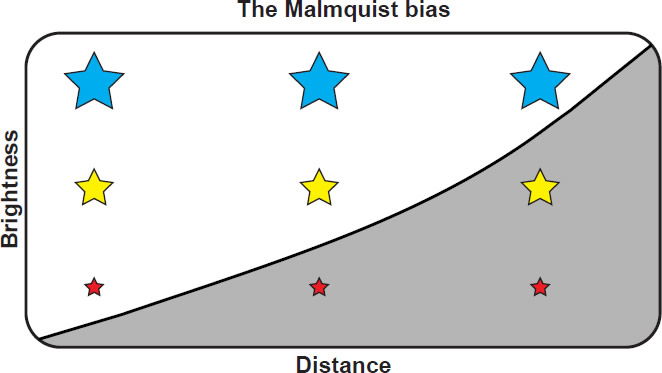
Fig. 1. Simplified illustration of the Malmquist bias. Bright blue stars can be detected at all distances in this survey, but the faint red stars can only be detected nearby. Hence, bright stars are overrepresented in magnitude-limited surveys.

This method is used without complication in surveys of stars; but in cosmic-scale surveys some additional caveats arise from the relativistic curvature of spacetime due to the mass, energy, and expansion of the universe. For example, in an expanding universe the intensity of light departs somewhat from the inverse square law. Such effects are negligible in our solar neighborhood, but the departure becomes very substantial at high redshift. Fortunately, these effects have been well studied, and there is a straightforward way to deal with them without having to explicitly work through the Einstein field equations. Namely, there are several different ways of defining distance, in order to deal with relativistic effects. We need mention only two: co-moving distance and luminosity distance.

Co-moving distance is defined using a non-static coordinate system that expands at exactly the same rate as the universe. Thus, when using co-moving coordinates, it is as if there is no expansion and the average density of the universe does not change with time. This coordinate system is therefore the most natural to use in geometric computations such as volume. For example, assuming that the cosmos is at least approximately homogeneous, the number density of galaxies is expected to be roughly independent of redshift only when volumes are computed in co-moving coordinates.

Luminosity distance is defined in such a way as to preserve the inverse-square law. That is, the intensity of light falls off as the inverse of the luminosity distance squared, by definition. This coordinate system is the most natural to use when dealing with magnitudes/brightnesses of galaxies. Luminosity distance is, in general, not the same as co-moving distance. However, they are similar at low redshift and converge in the limit as distance goes to zero. Given the cosmological parameters7 there are formulae available in standard cosmology textbooks to compute either type of distance from a given redshift.

Given this caveat, all methods of dealing with the Malmquist bias must use luminosity distances when computing limiting distances from apparent brightness under the inverse square law, and co-moving distance when computing volumes to estimate number density. For instance, in the volume-weighting method each galaxy is weighted by the inverse of the co-moving volume of space corresponding to the luminosity distance at which the galaxy could have been detected, given the limiting magnitude and range of the survey. It is often convenient to express the luminosity distance in terms of its corresponding distance modulus (μ) because the latter is logarithmic in the same way that magnitudes are. The distance modulus is defined to be the difference between apparent and absolute magnitude.

When distance modus is known, the apparent magnitude of a galaxy can be computed from its absolute magnitude, or vice versa. The distance of an object is related to the distance modulus by the following conversion:

where d_L is the luminosity distance in parsecs.

Though conceptually simple and computationally fast, there are drawbacks to using the volume weighting method against other methods. For one, our results suggest that, of the traditional methods, volume weighting is the most easily biased to errors in what is known as the K-correction—a caveat that we discuss below. The Lynden-Bell-Choloniewski method, which we discuss at length in other papers (Hebert and Lisle 2016a, b), fares better but still fails to completely remove the Malmquist bias.

These traditional methods tacitly assume that the limiting magnitude is a sharp cutoff—that the survey includes all galaxies brighter than this limiting magnitude and excludes all fainter galaxies. This is an unlikely scenario because the galaxies that are chosen to be included in a particular survey are selected for a variety of reasons beyond merely the limiting magnitude. As one example, galaxies are extended objects and so their detectability is also influenced by their surface brightness, the brightness per square arc second. Two galaxies of equal apparent magnitude may have very different surface brightnesses, so one may be detected while the other is lost.

The Target Function

To be included in the spectroscopic analysis (which includes redshift/distance estimations) of the Sloan Digital Sky Survey, a galaxy must be sufficiently bright to obtain a reliable spectrum. The SDSS target selection algorithm therefore rejects galaxies that have a Petrosian apparent magnitude higher (fainter) than 17.77 in the r-band (Strauss et al. 2002).8^,9 And so it seems most natural to use this number as the limiting magnitude for the survey when implementing the volume-weighting method or the Lynden-Bell-Choloniewski method.

We define the target function [T_S(m)] to be the probability that a galaxy of apparent magnitude (m) will be selected for spectroscopic analysis and inclusion in the main survey of SDSS. The target function is similar conceptually to the selection function. Both functions assess the fraction of galaxies that we are able to detect compared to the number of galaxies that actually exist. But the selection function is this fraction as a function of distance—the number of galaxies we can detect at a given distance divided by the number that exist at that distance. The target function is a function of apparent magnitude—the number of galaxies we can detect at a given apparent magnitude compared to the actual number of galaxies that exist at that apparent magnitude.

Naïvely, we might assume that the target function is a simple Heaviside step function; zero for apparent magnitudes above (fainter than) the limiting magnitude, and one for those below, as in Fig. 2. And in fact, all the above methods for estimating the luminosity and selection functions tacitly assume this. But in reality, the target function is not so simple for several reasons.

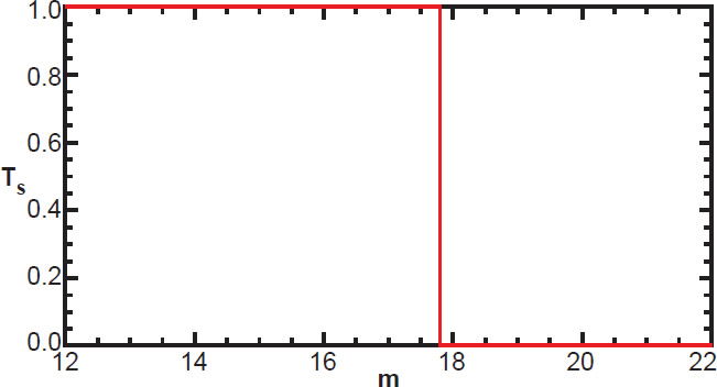
Fig. 2. The (incorrect) target function implicitly assumed in traditional methods.

First, the best estimate for the actual apparent magnitude (called the c-model apparent magnitude) of a galaxy is not exactly equal to its Petrosian magnitude. The difference between these two magnitudes is slight for any given galaxy. Yet there are some galaxies slightly fainter than apparent c-model magnitude 17.77 (in r-band) that are nonetheless included in the survey since their Petrosian magnitude is slightly brighter than 17.77, and vice versa. So rather than jumping instantly from unity to zero at m = 17.77, the target function is expected to transition more smoothly, with galaxy magnitudes near 17.77 having an intermediate probability of detection as shown in Fig. 3. This figure shows the actual target function derived from SDSS data by the method discussed below.

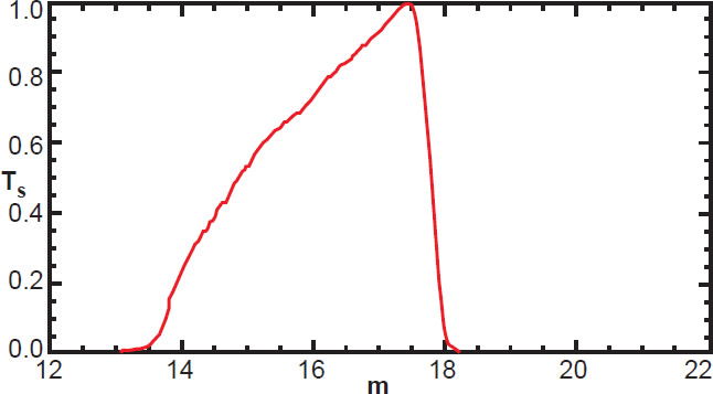
Fig. 3. The true target function in the c-model r-band for SDSS galaxies in our survey.

Second, there are additional criteria that galaxies must meet to be included in SDSS spectroscopic analysis. These are discussed in detail in Strauss et al. (2002), and we will briefly mention a few here. For example, a galaxy may be brighter than m = 17.77, and yet have a surface brightness too faint to record a reliable spectrum. Therefore, the SDSS algorithm rejects galaxies whose Petrosian surface brightness is fainter than 24.5 magnitude per square arc second.

Third, and perhaps counterintuitively, some galaxies are too bright to be included. A galaxy with very high surface brightness can saturate the detector, preventing accurate data analysis. Such galaxies are necessarily excluded from the spectroscopic survey. So we expect the target function to drop to zero at very low magnitudes, corresponding to very bright galaxies. Since galaxies vary greatly in size, there is not a one-to-one correspondence between overall brightness and surface brightness, the latter of which is more relevant to detector saturation. Thus, the target function tapers off gradually at low magnitudes, as shown on the left side of Fig. 3.

Fourth, we must consider the effect of contamination from nearby, bright, interloping sources such as stars, nebulae, and other galaxies. These contribute flux, increasing the initial brightness estimate of a galaxy, so that the estimated magnitude is more negative than the true magnitude. Although the SDSS algorithm estimates the contribution of foreground contamination, and removes such from final estimates of galaxy apparent magnitudes, the 17.77 cut is applied before such corrections are made. Therefore, a small fraction of galaxies whose actual r-band apparent magnitude is much larger (fainter) than 17.77, are nonetheless included in the survey because foreground contamination caused their initial observed apparent magnitude to be lower (brighter) than 17.77. And so the target function can have low, but non-zero values well above 17.77 as shown in Fig. 3. Neither the volume-weighting method nor the Lynden-Bell-Choloniewski method have any way of dealing with these low-brightness galaxies; they would have negative weight in the volume-weighting method (since they lie outside the volume at which they theoretically could have been detected), and they cannot be processed under the LBC method.

Fifth, some galaxies in the SDSS have been selected by a different survey criterion. The luminous red galaxy (LRG) survey selects galaxies based on color as measured in different filter sets. Since the LRG survey is not magnitude limited (within the limits imposed in our survey), it does not suffer from the Malmquist bias. Therefore, we have not included galaxies selected by the LRG survey unless they are also included in the primary survey. Only a small fraction of galaxies in our distance range are LRGs.

It is therefore desirable to use a method in which the true target function is used to compute the luminosity function and then the resulting selection function, as this would be more accurate than traditional methods. Unfortunately, the target function is not known in advance. However, it is possible to extract the target function and luminosity function simultaneously from the data by the method shown below.

Consider a subset of our data: the galaxies contained within a thin spherical shell whose radius is some distance modulus μ and whose thickness is Δμ. Fig. 4 shows a histogram of the absolute magnitudes of galaxies observed in our survey at various distances. Notice that the shape of the histogram depends on the distance modulus we select. As μ increases to larger distances, the distribution of observed galaxies shifts to brighter galaxies (lower absolute magnitudes). This is due to the Malmquist bias.

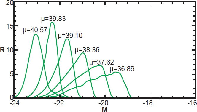
Fig. 4. R(M) at various distance moduli, normalized by area.

Presumably, the actual luminosity function does not change substantially with distance. (If it did, then efforts to obtain a luminosity function over the volume of the survey would be inaccurate and strongly biased toward the luminosity function of nearby galaxies.) Rather, our ability to detect bright or faint galaxies changes with distance since the target function depends on apparent magnitude. At any given distance modulus (μ) the histogram of galaxies we observe as a function of absolute magnitude R(M) will be the product of the true density of galaxies as a function of absolute magnitude (the luminosity function) times the fraction that can be detected (the target function). So we have:

The equation is an approximation because we have defined T_S to be a function of m only, regardless of distance, and it is not strictly true that detectability depends only on apparent magnitude for the reasons listed above, though it is the primary criterion. We are here presuming that the detected number of galaxies really is approximately equal to the product of two functions, one that depends only on absolute magnitude and the other only on apparent magnitude. We can test the accuracy of this approximation after its use, as described in the section entitled “The K Correction.” By construction, the target function is dependent only on apparent magnitude; but for a given distance modulus (μ) the apparent magnitude is the same as the absolute magnitude plus a constant, where that constant is the distance modulus: μ.

That is, the target function can be expressed in terms of absolute magnitude at a given distance. If we then change to a different distance, the shape of the curve remains unchanged, but its horizontal position is shifted by a constant. And since we are considering only a subset of galaxies that have the same distance modulus μ, the target function, expressed as a function of absolute magnitudes, will have the same horizontal offset μ for all these galaxies. So, for a given distance modulus μ, the observed number density of galaxies as a function of magnitude is:

The functional form of both Φ(M) and T_S(m) are not yet known. But all the other variables are known. We have distance information on each galaxy in the survey; the redshifts are known, and these can be used to compute an estimate of the distance modulus for every galaxy.10 The absolute magnitudes can then be computed from the observed apparent magnitudes by subtracting the distance modulus. So, for each galaxy, we know m, M, and μ. And we also know R: the density of observed galaxies of any given absolute magnitude within a spherical shell at distance modulus μ. This is found by simply counting the observed number of galaxies between μ and μ + Δμ, and dividing that number by the co-moving volume of that shell. So, R(M) is known for each distance modulus as illustrated in Fig. 4.

Since R(M) is a one-dimensional function of M for a given value of μ, when we consider all values of μ in our survey, R can be thought of as a two dimensional function R(M, μ). Here, R(M, μ) is the number density of galaxies with absolute magnitude between M and M + ΔM, and with distance modulus between μ and μ + Δμ, as depicted in Fig. 5. The grid shows lines of constant M and constant μ. Individual bins are not shown here, but are comparable to the thickness of the lines. We can pick a distance modulus range, μ_n to μ_n + Δμ (where Δμ is the height of a bin), as indicated by the green line, and plot R versus M for that selected value of μ_n. By iterating through a range of values of μ_n, we generate a sequence of curves, each of which is the observed number density of galaxies versus absolute magnitude at a given distance modulus as shown in Fig. 4. So each graph in Fig. 4 represents a horizontal slice of constant μ through R(M, μ).

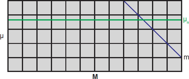
Fig. 5. Range of observed number density of galaxies. R(M, μ).

Consistent with previous studies, we expect that the luminosity function does not change substantially with distance, at least not until very high redshifts. And so to high accuracy, the luminosity function depends only on M, not on μ. And, by definition, the target function depends only on apparent magnitude (m) which is absolute magnitude plus distance modulus (M + μ). Since the apparent magnitude is the primary criteria by which galaxies are selected for inclusion in the survey, we expect that the target function will not change shape significantly with distance; it merely shifts leftward with increasing μ. For the moment, we limit our investigation to low redshifts where the K-correction (to be discussed later) is small. We now have

That is, we have a two-dimensional function expressed as a product of two one-dimensional functions. The two dimensional function R(M, μ) is known for the range of M and μ in the survey. Our goal is to find the functional forms of Φ(M) and T_S (M + μ) such that when these two functions are multiplied, they result in the observed curve R(M) at any given distance modulus. There are several possible ways to do this. We will now cover one such method that is intuitive and computationally fast.

The Method

It is natural to think of absolute magnitude and distance modulus as two independent quantities, where apparent magnitude is their sum (Fig. 5). In such a view, R(M, μ) is a rectangular array, with the x-axis representing absolute magnitude and the y-axis indicating distance modulus. Positive is up and right for each axis respectively, which means that the brightest galaxies will be on the left side of R. Lines of constant apparent magnitude occur on the diagonals, with a slope of negative one, as shown in blue on Fig. 5.

For our purposes it is conceptually better to think of absolute magnitude and apparent magnitude as independent quantities with distance modulus being a function dependent on their difference. Visually, this is a sheared version of Fig. 5, as shown in Fig. 6. The x-axis represents absolute magnitude as before, but the y-axis now represents apparent magnitude. Lines of constant distance modulus are now diagonal with a slope of positive one. The selected range of our survey, where R(M, m) is known, is the gray parallelogram. Plotted this way, Φ(M) and T_S(m) are now functions of orthogonal coordinates.

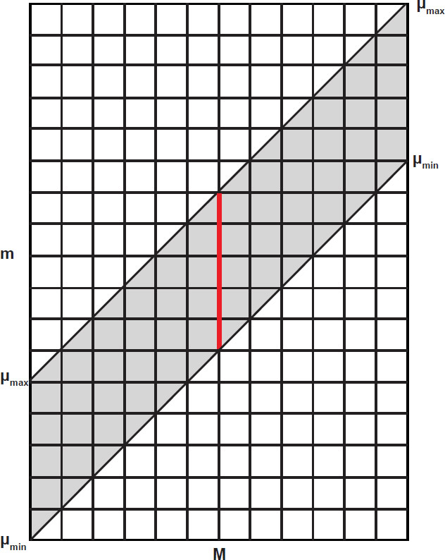
Fig. 6. Range of observed galaxy density as a function of M and m.

For any given M (such as the red column of bins in Fig. 6), the luminosity function is a constant that does not change with distance modus or apparent magnitude. Hence, any variation in R as we move along this red segment must be due solely to the functional form of T_S(m). Conversely, T_S(m) does not vary along lines of constant m; any variation in R value along horizontal lines is due solely to the form of the luminosity function. We can think of R as the product of two orthogonal functions where T_S(m) alone is responsible for any variation in R along the y-axis, and Φ(M) alone is responsible for any variation along the x-axis. It is possible to deconvolve the contributions of T_S(m) and Φ(M) by considering how values of R(M, m) change as we move along each axis.

Fig. 7 illustrates the data bins of R(M, m). Each bin has width ΔM and height Δm. To estimate Φ(M) we select a value of M within our data range. The choice of M does not matter, as long as it corresponds to a part of our survey where we have a reasonably high galaxy count (i.e., not near the edges). The selected magnitude will correspond to a particular column (particular value of n) of R(M, m). We then take the sum value (S_n) of all R(M, m) in column n, with the exception of the bottom bin as shown in Fig. 7. We define S_n to be the sum of all values of R(M, m) in column n excluding the lowest bin.

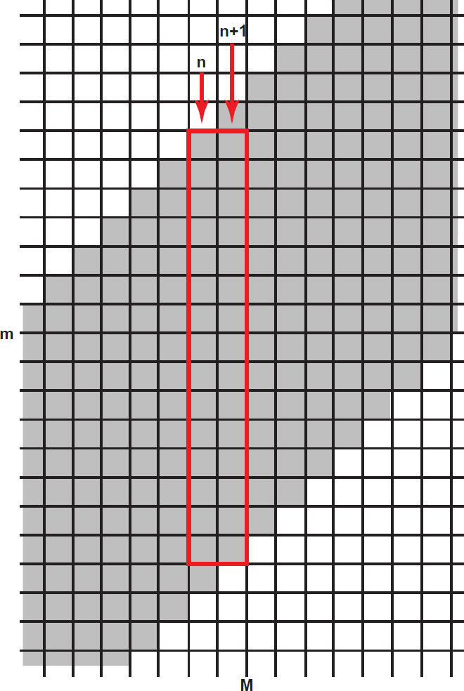
Fig. 7. A section of R(M,m) showing individual data bins.

Next, we move one column to the right and take the sum (U_n+1) of all values of R(M, m) except the top bin in column n+1. Here, we have defined U_n as the sum of all values of R(M, m) in column n except the top bin. When we compare S_n with U_n+1, (see the red box in Fig. 7) they will not, in general, have the same value. Any difference between the two cannot be due to any change in T_S(m), because the value of m has not changed. Thus, any difference between S_n and U_n+1 must be due to the difference in Φ(M) at n and n+1 respectively since only M has changed.

It follows that

We now have Φ(M + ΔM) in terms of Φ(M). We then move on to the next column, n+2. This time, we compare U_n+2 with S_n+1. Since we have excluded the lowest bin in the n + 1 column, and the topmost bin in the n + 2 column, we are again looking at changes of R(M, m) in the horizontal direction only. Again, this change must be due solely to the change in Φ(M) since m remains constant. We now have the ratio of Φ(M + 2ΔM) to Φ(M + ΔM). And since we previously obtained Φ(M + ΔM/Φ(M), we can get Φ(M + 2ΔM) in terms of Φ(M). We continue this process until we reach either a column whose sum is zero, or the edge of our range. We can also go in the reverse direction, finding the relative values of Φ for n–1, n–2, etc. When completed, we have the luminosity function for all values of M in terms of the value of Φ(M) at our starting M. That is, we have the luminosity function times an unknown constant. That constant will be found later when the function is normalized.

Note that we can, in principle, estimate Φ(M + ΔM)/ Φ(M) by comparing just two bins in the same row. But this would make use of only a small fraction of our data. By comparing S_n and U_n+1 we get much higher signal to noise. Since the columns are typically over 100 bins in height, and since we exclude only one bin in each column during our comparison, this method uses over 99% of the data in each column at each step.

Since we have Φ(M) (times a constant) for all M, and since we know R(M, m), we can find T_S(m) (also times a constant) for all m.

T_S could be estimated for each value of R(M, m), and then averaged across a row to get the estimate of T_S(m) for any given m, but this would give equal weight to each bin even though some may have very low data counts. Greater accuracy is obtained if the bins are weighted proportionally to the luminosity function at the given value of M. This is accomplished for any selected value of m, by first summing over all values of R(M, m) in that row, and then dividing by the sum of the luminosity function over the same range (from M₀ to M₁). For any given m, this is:

This effectively gives more weight to regions where the luminosity function (and thus the detected galaxy count) is higher, thereby reducing the effects of noise in data bins with low galaxy count.

Once the form of T_S(m) has been determined, we can normalize both it and the luminosity function by assuming that the highest value of T_S(m) is one. Clearly, T_S(m) can never be higher than unity, because it represents the probability of detection.

The target function might never reach unity at any point, because there may be some galaxies that cannot be detected even at its optimal apparent magnitude—too close to a star, unusual appearance making galaxy classification difficult, etc. But we expect these would not be common. So normalizing T_S(m) to have a maximum of 1 is a good approximation. Once T_S(m) is normalized, the luminosity function can be normalized as well since it is inversely related to T_S(m) by our data R(M, m).

Note that the above method of determining Φ(M) only works until we reach a column whose sum is zero. Using this method in such a case would yield Φ(M) equal to zero for such a column. Any columns thereafter cannot be determined as a ratio to Φ(M) without dividing by zero. However, with a slight modification to the method, Φ(M) for such columns can be determined. We can “skip” a column of zeros (at n + 1) by comparing the sum of values of R(M, m) at n (obtained by excluding the bottom two bins in the nth column) with the sum of values at n + 2 (obtained by excluding the top two bins in column number n + 2). Since the shift is again horizontal only, it follows that Φ(M + 2ΔM/ Φ(M) must equal the ratio of these two sums. However, since we expect the luminosity function would not go to zero and then come up again, such modification to the method is not expected to be necessary. If a column near the edge of the data range does go to zero, data beyond this point are of sufficiently low signal-to-noise to be ignored. If a column of zeros occurs far from the edge of the data range, this suggests that the data range has not been appropriately selected, or that the chosen bin size is far too small.

Algorithm Parameters

Since both Φ(M) and T_S(m) are expected to be smooth functions, it may be helpful to apply a small amount of smoothing (averaging each array element with the surrounding values) to the resulting luminosity function in order to reduce the noise caused by small numbers of galaxies in a given bin. The amount of smoothing will depend on the number of absolute magnitude bins, with higher resolution requiring more smoothing due to the fact that fewer galaxies will fall into a given bin. With an absolute magnitude range of 8, we found 300 bins with a smoothing of 5 to 10 bins resulted in a reasonably smooth luminosity function. The results were not significantly affected by higher values (greater number of bins) of smoothing. Since the method works for any reasonable bin size, the choice of bin size is determined by the trade-off between resolution and signal-to-noise ratio.

The above method requires that bins of R(M, m) are square: the bins must have the same height in apparent magnitude as width in absolute magnitude so that the data limits have a slope of positive one (see Figs. 6 and 7). This is necessary so that we can properly compare S_n and U_n+1 directly without having to estimate the value of a fraction of a bin.

The number of absolute magnitude bins (h) used for computing the luminosity function may be freely chosen—we used 300. Choosing a greater numbers of bins increases resolution at the expense of signal-to-noise in any one bin. But once this number has been chosen, it will determine the number of bins (v) of apparent magnitude for the target function necessary to use all our data, based on the distance range used in the survey, and the absolute magnitude range we are considering. This is due to the aforementioned requirement that the bins must be square. We compute this vertical number of bins in two steps.

First, we find the number of “distance bins”—that is the number of bins in a single column that have data, since they are within range of the survey, (as in the red line in Fig. 6). In Fig. 7 this is illustrated as 16 bins (though the actual value from our survey is much larger); each column has 16 shaded bins, indicating bins that contain data. The number of distance bins will be the number of magnitude bins (h) multiplied by the distance modulus difference (μ_max–μ_min) and divided by the absolute magnitude difference (M_max–M_min).

Second, we add this number of distance bins to the number of absolute magnitude bins, and subtract one (since distances are from bin center to the next bin center). So the number of vertical bins (v) relates to the number of horizontal bins (h) by:

We note that this method is predicated upon the assumptions that the luminosity function does not change appreciably with distance, and that the target function is dependent only on apparent magnitude. The second criterion is not strictly true, but is reasonable as a statistical trend for SDSS galaxies obtained in the main (Legacy) survey. It may be possible to obtain even higher accuracy for the luminosity function by relaxing this condition and allowing T_S to vary smoothly with distance and estimating its form at multiple distances from the luminosity function computed from the initial pass.

The K-Correction

If galaxies were not redshifted and their distances could be determined by some other means, then no additional corrections would be necessary. But since the SDSS survey measures the flux of a galaxy within certain filter bands, we must consider what effect redshift has on estimates of absolute magnitude.

If a galaxy had no redshift, then its absolute magnitude in a particular filter band would be the apparent magnitude in that band minus the distance modulus. But consider a second galaxy of identical spectrum and absolute magnitude to the first, but with some positive redshift. Since this galaxy’s spectral features are redshifted, some of the longer wavelengths that were within the filter band for the first galaxy have been shifted out of range—resulting in a drop in detected flux. On the other hand, some of the shorter wavelengths that were beyond the filter range for the first galaxy have now been shifted into this range for the redshifted galaxy—resulting in an increase in detected flux. Depending on the slope of the spectrum of the galaxy, one of these two effects will generally be stronger than the other. Thus, its apparent magnitude in a given filter will not be simply the absolute magnitude plus the distance modulus.

So, when computing the absolute magnitude of a redshifted galaxy from its apparent magnitude in a particular filter band, it is necessary for us to introduce a correction to compensate for the shift of a galaxy’s spectrum from the rest frame with respect to the bandpass filter: the K-correction.

Since K depends on the bandpass filter, the spectrum of a galaxy, and the redshift, it will differ from one galaxy to another, and from one filter set to another. Note that the K-correction would be unnecessary if we could somehow measure all of a galaxy’s flux across the entire electromagnetic spectrum. A discussion of the K-correction is provided in Hogg et al. (2002).

In principle, it is possible to compute the K-correction exactly for each galaxy whose spectrum is known. But this would involve obtaining the spectrum for each of the 600,000+ galaxies in the survey and shifting their spectrum through the response function of the given bandpass filter, including for atmospheric extinction, which would be tedious. Fortunately, the K-correction has been well-studied and there are computationally efficient means of approximating it with high accuracy given only (1) the redshift of the galaxy, (2) the galaxy’s color (the difference in magnitude as observed between two different filters), and (3) the selected filters. The K-correction is well-approximated by a fifth-order polynomial whose parameters are known for the SDSS filter sets (Chilingarian, Melchior, and Zolotukhin 2010). We have used this method so that all our absolute magnitude estimates are K-corrected.

The Inverse K-Correction

Only the standard K-correction is necessary to compute the correct absolute magnitude of each galaxy in a survey. But if we want to compute the luminosity function and selection function by any method, we must use the target function or its equivalent to estimate how many unobserved galaxies exist for each observed galaxy of a given absolute magnitude. But the target function depends on the apparent magnitude of any given galaxy, and apparent magnitudes are not K-corrected. The traditional methods ignore this important subtlety. Yet it results in a bias in both the luminosity function and the selection function. This is easiest to explain with the volume-weighting method.

In the volume-weighting method, we find the K-corrected absolute magnitude of each galaxy from its apparent magnitude, distance modulus, and K-correction. Then each galaxy is weighted by the inverse of the co-moving volume corresponding to the minimum and maximum distances in which the galaxy could have been detected and included in the survey. The maximum distance is determined by the limiting magnitude of the survey (17.77 in r-band for the SDSS survey).11 Normally, this is found by solving for the distance modulus at which the apparent magnitude of the galaxy equals the limiting magnitude of the survey. That is, we set m_lim = M + μ_max and solve for μ_max. But this is not exactly true because it ignores the K-correction, and therefore the galaxy weighting will be inaccurate. (The effect is small for low redshifts, but becomes significant for galaxies near the upper limit of our analysis.) The actual relationship between the limiting magnitude and the true absolute magnitude is:

Here, K_lim is the K-correction that the galaxy would have at that limiting distance. Unfortunately, this is unknown, and very difficult to estimate. We have previously computed the K-correction that each galaxy has at its actual distance. But this is not equal to the K-correction that the galaxy would have if placed at its limiting distance, because the K-correction depends on both redshift and the apparent (redshifted) color of a galaxy at its true distance. To find the limiting distance, we must perform an inverse K-correction. That is, we must estimate what the K-correction would be for a galaxy whose absolute magnitude is known if that galaxy were placed at the maximum distance at which it could be detected.

The inverse K-correction is very difficult to compute from the aforementioned approximation and has multiple solutions for a given galaxy. Fortunately, the K-correction is relatively small for our redshift range, and therefore its inverse will be small as well. So an approximation of the inverse K-correction is sufficient to obtain an accurate luminosity function and selection function. There are perhaps many ways to do this. The following method is computationally efficient and gives accurate results.

Rather than attempting to invert the K-correction on a per-galaxy basis, we instead find the average K-correction as a function of distance modulus for all galaxies within our survey. We find this by plotting the known K-correction for all galaxies in our survey, and find the average value for a given distance modulus, as shown in Fig. 8. The resulting curve is well-described by a cubic function:

This function will serve as an approximation of the K-correction for a given redshift. For the SDSS main survey galaxies between 0.05 and 0.28, the best-fit parameters are A = 8.127 × 10^-4, B = 0.02113, C = 0.09287, D = 0.1346. Since this function has a positive slope everywhere in our data range, its inverse has only one solution (distance modulus) for a given value of K. Thus, finding the inverse K-correction and limiting distance of a galaxy from its absolute magnitude is straightforward.

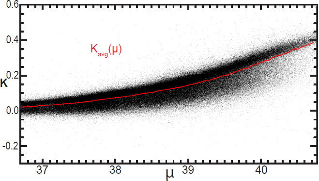
Fig. 8. The K-correction of all SDSS main survey galaxies as a function of distance modulus, with the average K-correction at each distance shown in red.

Note that the true K-correction depends on both redshift and galaxy color, whereas our approximation depends only on redshift. Also, note that this approximation is only needed when finding the inverse of the K-correction. All absolute magnitude estimates in our survey are based on the more accurate forward K-correction. The inverted form is only needed to determine how galaxies should be weighted in their contribution to the luminosity function.

Similarly, with both the Lynden-Bell-Choloniewski method and the new method introduced in this paper, this average K-correction can be used to reduce bias in the luminosity function. Both methods tacitly assume that m = M + μ with no K-correction when computing the luminosity function. The LBC method does this when it imposes the limiting magnitude cutoff as a function of M and μ only (see Hebert and Lisle 2016a,b). The new method does this by computing which apparent magnitude bin the galaxy should be placed in based on its distance modulus and absolute magnitude. A simple workaround is to define a new parameter:

This new “modified distance modulus” (μ_K) includes the average K-correction of galaxies at the corresponding distance. Since we have defined K_avg such that on average, m = M + μ + K_avg it follows that:

Although this equation is only approximate for any given galaxy, we expect it to be highly accurate when we consider the sum of all the galaxies since it is based on the average K-correction for our survey. By converting all distances to this modified distance modulus μ_K, we can proceed (with either the LBC method or the new method) as if there were no K-correction. After the selection function is computed in terms of μ_K, we can convert the distances back to μ to obtain the selection function as a function of actual distance. The results shown below make use of this correction.

Evaluating the Resulting Luminosity Function

The luminosity function resulting from our analysis of approximately 600,000 galaxies between redshifts of 0.05 and 0.28 is shown in Fig. 9 on a logarithmic scale. The target function resulting from our analysis is shown in Fig. 3. We can estimate the correctness of both of these curves by seeing if their product at a given distance modulus closely matches the curve of observed galaxy density R(M) at that same modulus.

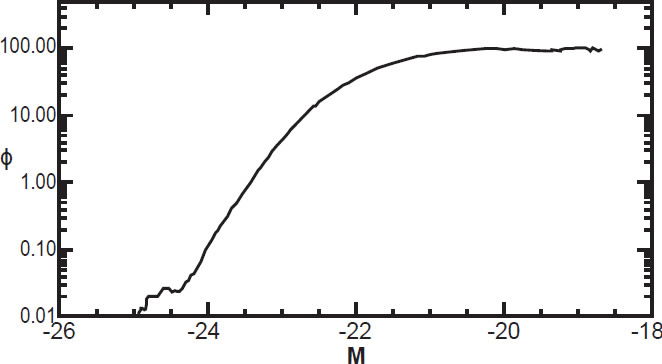
Fig. 9. The luminosity function for SDSS legacy survey.

It may seem at first that they would have to, since they were derived under this very assumption. But this is not so. There is no guarantee that R(M, μ) actually can be well approximated as the product of two one-dimensional functions, one depending only on M with the other depending only on m. No doubt our algorithm ensures that the product of Φ(M) and T_S(m) is a best fit to R(M, μ). But there is no guarantee that the best fit is a good fit.

The ability of the product of Φ(M) and T_S(m) to reproduce R(M, μ) will be a good test of our initial assumption that T_S(m) really does depend only on m, and that Φ(M) really does not change appreciably with distance. Fig. 10 illustrates this comparison with the green curves showing R(M) at two different values of μ, and blue curves showing the product of Φ(M) and T_S(m + m) at those same values of μ. The curves are normalized to have the same area so that both can be visualized on the same graph. The fit is remarkable, suggesting that we indeed have a very accurate estimate of both the luminosity function and target function.

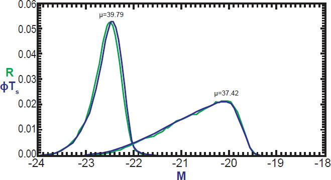
Fig. 10. Comparison of data (green) and best fit Φ(M) T_S(M+μ) (blue).

The Selection Function

The selection function is the ratio of galaxies detected to total galaxies at a given redshift. We naturally expect that the selection function will decrease with increasing z, since galaxies become harder to detect at increasing distance. Nonetheless, the selection function will not be unity even at very close distances, since some nearby galaxies are too bright to be included in the SDSS survey. The selection function is expressed mathematically as:

where μ is the distance modulus corresponding to redshift z. The exact relationship between z and μ will depend on the chosen cosmological parameters. Given a value of z one can compute the value of μ directly, and vice versa. Since the target function and luminosity function are now both known, computing the selection function is straightforward.

As a matter of practicality, the selection function tells us the fraction of galaxies we are detecting above a particular threshold luminosity. This limitation is imposed because we do not know the luminosity function over an infinite range. The upper limit on magnitude is set by the limiting apparent magnitude of the survey instruments combined with the minimum distance of our survey. In our case, the luminosity function is well-determined at absolute magnitudes below –19. This corresponds roughly to the limiting apparent magnitude for the nearest galaxies in our survey.

Note that traditional methods cannot determine anything about galaxies fainter than this cutoff, since they implicitly assume that the target function is zero for galaxies fainter than the cutoff value. The method presented in this paper is able to go several magnitudes fainter, up to nearly –16, since the target function is non-zero for several magnitudes above the theoretically expected limit. However, since these data points are in the tail of the target function, their reliability is suspect. We therefore truncate the luminosity function at M = –19 when computing the selection function. The resulting selection function is plotted in Fig. 11. This tells us the fraction of galaxies included in the survey at a given distance divided by the true number whose absolute magnitude is less than –19.

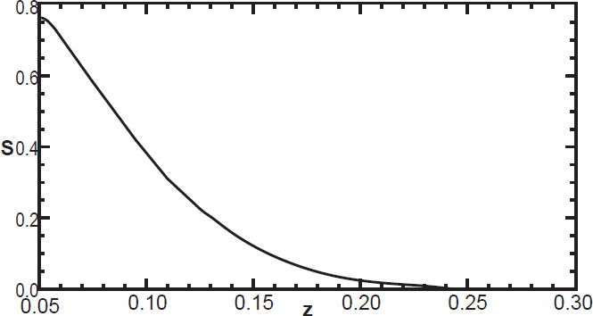
Fig. 11. The selection function for M ≤ –19.

At redshift of 0.05, we are detecting 76% of galaxies brighter than M = –19. By redshift z = 0.15, we are capturing only 13% of the galaxies. And at z = 0.28, we are capturing only 0.15% of galaxies brighter than M = –19.

Results and Comparison with Traditional Methods

We compare the resulting luminosity function of our method with that obtained by the volume weighting method and Lynden-Bell-Choloniewski method in Fig. 12. All these methods use the same data. All absolute magnitudes have been K-corrected. The results from the standard volume weighting method and LBC method are shown in pink and green respectively. These methods do not account for the inverse K-correction. We also consider the results of these methods using the modified distance modulus, which takes account of the average (inverse) K-correction, shown in red for volume weighting and blue for LBC.

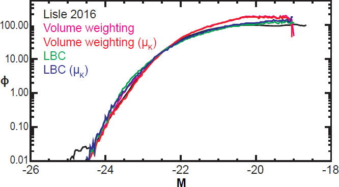
Fig. 12. The luminosity function as estimated by various methods.

For ease of comparison, the methods are normalized to have the same value at M = –22.5. All methods show general agreement, though the volume weighting method gives higher estimates of low-brightness galaxies. The traditional methods lose precision (and volume weighting loses accuracy as well) for the highest magnitude (faintest) galaxies, whereas the new method gives reasonable estimates even slightly above the theoretical detection threshold of –19. The new method reports higher values for the very brightest galaxies at M < –24.5, though these data have very low signal to noise. Conversely, it gives much more reliable estimates of low-luminosity galaxies, which is far more important in determining the selection function since the faintest galaxies outnumber the brightest ones by four orders of magnitude. For this reason and also because the new method attempts to use the true target function rather than an arbitrarily chosen Heaviside function, we expect the method presented here to result in a more accurate selection function than other methods produce. This is confirmed by the flatness of the plot of galaxy number density as a function of co-moving distance (Fig. 13).

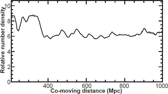
Fig. 13. The relative number density of galaxies as a function of distance from earth in megaparsecs.

Fig. 13 shows that the number density of galaxies is relatively constant as a function of distance, aside from small scale perturbations and a larger concentration at 200 < d_C < 350 megaparsecs. This plot is a histogram of observed SDSS main survey galaxies divided by the selection function as estimated from the method described above. Since galaxy density is expected to be roughly constant with co-moving distance, the flatness of this plot implies that our selection function is accurate.

This expected flatness also implies (but does not prove) that the standard estimates of the cosmological parameters are basically correct. This is because the relationship between the measured luminosity distance and the computed co-moving distance is strongly dependent on these parameters, particularly at large distances. So, the overall flatness of Fig. 13 is consistent with the current best estimates of the Hubble constant, dark matter, the cosmological constant, and the assumption of homogeneity. However, this does not preclude the possibility that a different set of cosmological parameters and assumptions might also result in a flat number density plot.

Note that our selection function (as shown in Fig. 11) is smooth; it shows no local maxima but is everywhere negatively sloped. This is also the case with the selection functions derived by the volume weighting and LBC methods respectively. Since the selection function is smooth, this implies that the local maxima in Fig. 13 are real in redshift space; they are not an artifact of the way the SDSS data were collected. The distances at which we find notable greater-than-average density occur at 323, 473, 551, 616, 677, 737, and 902 Mpc.

Note that the local over-densities are small. Therefore, if the quantization effect is real it is not strong but rather a weak trend. Further study will be required in order to determine if these peaks are statistically significant. Whether they genuinely represent concentric shells, or are merely due to random cosmic variance is yet to be determined. Moreover, the possibility that such apparent over-densities are due to the conversion from redshift to distance must be considered. This is because redshift is used as a proxy for distance, yet redshift depends on both cosmic distance (called Hubble flow) and the motion of a galaxy through space (called peculiar velocity). Thus, maps of cosmic structure in which redshifts are used as a proxy for distance can suffer from apparent observer-centered artifacts, such as the “fingers of God” structures. It has been suggested that the bulls-eye effect can be similarly explained, though this has not been rigorously demonstrated (Praton, Melott, and McKee 1997).

Conclusion

The removal of the Malmquist bias is a necessary and important step in the analysis of SDSS galaxy data. The new method of obtaining the luminosity, target, and selection functions introduced here is computationally efficient, and gives results that are reasonable and consistent. Results are consistent with the standard cosmological parameters. Small perturbations of galaxy density as a function of redshift are real, though small. The method developed here may be used for further study of SDSS data or data from other surveys.

References

Chilingarian, I., A. Melchior, and I. Zolotukhin. 2010. “Analytical Approximations of K-corrections in Optical and Near-Infrared Bands.” Monthly Notices of the Royal Astronomical Society 405 (3): 1409–1420.

Choloniewski, J. 1986. “New Method for the Determination of the Luminosity Function of Galaxies.” Monthly Notices of the Royal Astronomical Society 223 (1): 1–9.

Choloniewski, J. 1987. “On Lynden-Bell’s Method for the Determination of the Luminosity Function.” Monthly Notices of the Royal Astronomical Society 226 (2): 273–280.

Efstathiou, G., R. S. Ellis, and B. A. Peterson. 1988. “Analysis of a Complete Galaxy Redshift Survey—II. The Field- Galaxy Luminosity Function.” Monthly Notices of the Royal Astronomical Society 232 (2): 431–461.

Hebert, J., and J. Lisle. 2016a. “A Review of the Lynden-Bell/ Choloniewski Method for Obtaining Galaxy Luminosity Functions: Part I.” Creation Research Society Quarterly in press.

Hebert, J., and J. Lisle. 2016b. “A Review of the Lynden-Bell/ Choloniewski Method for Obtaining Galaxy Luminosity Functions: Part II.” Creation Research Society Quarterly in press.

Hogg, D. W., I. K. Baldry, M. R. Blanton, and D. J. Eisenstein. 2002. “The K Correction.” http://ned.ipac.caltech.edu/level5/ Sept02/Hogg/paper.pdf.

Praton, E. A., A. L. Melott, and M. Q. McKee. 1997 “The Bull’s- Eye Effect: Are Galaxy Walls Observationally Enhanced?” The Astrophysical Journal Letters 479 (1): L15–L18.

Strauss, M. A., D. H. Weinberg, R. H. Lupton, V. K. Narayanan, J. Annis, M. Bernardi, M. Blanton, et al. 2002. “Spectroscopic Target Selection in the Sloan Digital Sky Survey: The Main Galaxy Sample.” The Astronomical Journal 124 (3): 1810– 1824.

Takeuchi, T. T. 2000. “Application of the Information Criterion to the Estimation of Galaxy Luminosity Function.” Astrophysics and Space Science 271 (3): 213–226.