The views expressed in this paper are those of the writer(s) and are not necessarily those of the ARJ Editor or Answers in Genesis.
Abstract
In his recently-published critiques, Reeves provides numerous important suggestions for the improvement of baraminology as well as pointed criticism of baraminic distance correlation (BDC). Given that BDC violates certain methodological assumptions, Reeves concludes that it is at best a heuristic of unknowable utility. Here, I evaluate 82 distance matrices taken from a previous study of Cenozoic mammals. After defining a BDC clustering method, I find that Pearson-based BDC performs as well as or better than medoid partitioning, fuzzy clustering, and Spearman-based BDC. The majority of Pearson BDC clusters (68.9%) also appear as clades in published phylogenies using the same character sets. I therefore conclude that despite questions about its formal validity, Pearson BDC remains a useful heuristic for clustering taxa and should not be rejected merely on the basis of Reeves’s critique. Because a large minority of studies revealed disagreement between different clustering methods, greater uncertainty about the previous baraminological conclusions was introduced using medoid partitioning and fuzzy clustering. Consequently, I recommend using multiple clustering techniques (Pearson BDC, Spearman BDC, fuzzy analysis, and medoid partitioning) in future baraminology studies.
Keywords: Baraminology, statistical baraminology, medoid partition, fuzzy clustering, Cenozoic mammals, created kinds
The theoretical concepts underlying the science of created kinds have been around since the time of Linnaeus. Though Linnaeus became known for species fixity, he softened his beliefs later in his career, suggesting instead that new species could indeed arise from previously-existing species. Darwin took this malleability of species and turned it into an over-reaching explanation for a vast array of biological and geological data, from the order of the fossil record to anatomical similarities to the adaptability of domesticated animals. In response, creationists asserted that biological change had limits. Frank Marsh frequently mentioned discontinuity, the created difference between kinds, or as he called them, baramins. “[A]lthough certain morphological structures do appear similar in many kinds, still a much more obvious phenomenon is the discontinuity between kinds” (Marsh 1944, 187).
While Marsh conceived of this discontinuity as a physiological limit of variation, modern statistical baraminology focuses on testing a “discontinuity hypothesis.” As previously described, “This is the research program of baraminology, to evaluate the claim that organisms were created in discrete, discontinuous groups that are recognizably different from all other organisms. We can call this idea the ‘discontinuity hypothesis’” (Wood 2011a). The principle test previously used to detect discontinuity is a combination of methodologies, which begin with the discrete character matrices that are found in published phylogenetic studies. Specifically, an n × n distance matrix is calculated using a simple matching coefficient referred to as a baraminic distance, where n is the number of taxa. Next, a matrix of linear correlation coefficients and probability estimates are calculated from the distance matrix by pairwise comparison of rows, yielding a baraminic distance correlation for each pair of taxa. BDC is more recently done using a standard bootstrapping of characters, in order to assess the sensitivity of the observed BDC patterns to perturbations in the underlying character matrix (Wood 2008a). Finally, a method of visualizing the distances using multidimensional scaling (MDS) or analysis of pattern (ANOPA) aids in the interpretation of the BDC (Cavanaugh and Sternberg 2002; Wood 2005a). These techniques have been applied to more than a hundred different character matrices (for example, Wood 2005b, 2008b; Thompson and Wood 2018).
In two extensive papers, Colin Reeves (2021a, 2021b) offers a substantive critique of the entire statistical baraminology program, from the simple matching coefficient as the distance of choice to the BDC and MDS techniques used to evaluate the distance matrix. As an alternative to BDC, Reeves offers a study of a turtle character matrix using two distance metrics (simple matching and Jaccard distances) and two clustering methods (medoid partitioning and fuzzy analysis). Having known about Reeves’s papers for several years, I am delighted to see them finally in print, and I and all creationists are immensely indebted to him for assisting us in placing the statistical analysis of baramins on a somewhat firmer foundation. While Reeves has made a valuable contribution to baraminology, his articles are not without shortcomings, which must be studied carefully to identify a practical way forward.
Here, I review the program of morphology-focused statistical baraminology and then evaluate Reeves’s claims regarding previous baraminology analyses. My intention is not to offer a simple rebuttal, but to clearly identify the problems and shortcomings of BDC in order to offer possible corrections. I then re-evaluate a selection of mammal baraminology studies from a recent publication (Thompson and Wood 2018). My results indicate that the methods recommended by Reeves produce results very similar to the original BDC studies, indicating that the methodology, though on questionable statistical foundations, nevertheless provides a very useful heuristic.
A Brief Review of Morphology-Based Baraminology
Before exploring new statistical baraminology techniques recommended by Reeves, it is valuable to review the objectives of statistical baraminology as I see them, because none of these change or ought to change in light of Reeves’s comments. In the 1990s, baraminology was still largely based around hybridization, as recommended by Frank Marsh (1944). Since so much of the creation/evolution debate focused on putative “transitional forms,” such as four-legged “whales” (e.g., Wieland 1990), the horse series (for example, Chapman 1991), and australopiths (for example, DuBois 1988), my colleagues and I desired a different, purely morphological method that we could use to interpret interesting fossil cases and other cases where hybridization was neither available nor practical.
In 2003, I and three colleagues introduced a “refined baramin concept,” which we described based entirely on similarity (Wood et al. 2003). The refined baramin concept summarized what we were trying to do with statistical baraminology as well as providing a guide for future research. The refined baramin concept explicitly endorsed similarity and dissimilarity as the defining characteristic of baramins, from which hypotheses of ancestry could be proposed and explored. This had the advantage of moving baraminology strictly into the empirical realm rather than untestable inferences of common ancestry.
According to the refined baramin concept, a holobaramin is “a group of known organisms that share continuity (that is, each member is continuous with at least one other member) and are bounded by discontinuity.” We defined continuity as significant, holistic similarity and discontinuity as significant, holistic difference. In practical terms, statistical baraminology studies do not achieve genuinely holistic analyses. Instead, “holistic” became a guide to selecting character matrices. For example, character matrices that included both cranial and postcranial characters were preferred over matrices of just cranial characters. Matrices of very limited scope, like dental characters only, were generally to be avoided. Likewise, character matrices with more characters were preferred to those with fewer, with the understanding that any sample of characters may or may not be a reliable reflection of all possible characters. Thus, the emphasis on “holistic” was not an attempt to make an empirical claim about the value or validity of certain character matrices but rather a philosophical guiding principle for selecting the sort of characters used in statistical baraminology. Indeed, without some independent knowledge of baramin boundaries, we cannot hope to empirically validate any set of characters, holistic or otherwise (or distance metrics, weighting schemes, or clustering techniques, for that matter).
In a more recent paper (Wood 2011a), I outlined the “discontinuity hypothesis,” which I still believe is an excellent goal for statistical baraminology. My explanation of the discontinuity hypothesis is worth quoting at length.
When we consider the biblical and biological evidence together, it seems quite reasonable to hypothesize that God created organisms in the categories that we call baramins, within which considerable diversification and speciation can take place but between which there are significant dissimilarities that Marsh called discontinuity. Though these conclusions are reasonable, as I explained above, they are not clearly and irrefutably taught in the Bible and are therefore open to empirical testing, insofar as we can do so. This is the research program of baraminology, to evaluate the claim that organisms were created in discrete, discontinuous groups that are recognizably different from all other organisms. We can call this idea the “discontinuity hypothesis”. (Wood 2011a)
The practicality of testing this hypothesis brings us to the question at hand: What is the best practice for detecting discontinuity?
Reeves chides me for considering only one sort of distance metric that may not be the best metric for the data available. This is certainly a fair concern, but Reeves spends little time discussing the quality of the character data to which the distance metrics are applied. His neglect of data quality is understandable, since he is concerned with the statistical validity of techniques applied to the character data, but if we are to proceed with statistical methods, we must consider strategies for measuring, assessing, and dealing with data quality.
For the typical character data used in previous statistical baraminology studies, the most conspicuous quality issue is the unknown character state. For example, Dembo et al.’s (2016) recent supermatrix for evaluating the phylogenetic position of Homo naledi contains 24 taxa and 391 characters for a total of 9,384 possible character states. Of those possible character states, only 4,774 (50.9%) are scored, and the unknown character states are unevenly distributed among the taxa. At least 74.9% of the character states are recorded for extant taxa (Homo sapiens, Pan troglodytes, and Gorilla gorilla), but the fragmentary remains of Kenyanthropus platyops are represented by only 37 (9.5%) recorded character states. Similarly, Australopithecus anamensis and A. garhi are represented by only 12.3% and 11.3% of the character states. Some missing character states could conceivably be discovered through a more careful examination of the presently-available fossils, but others cannot be known unless future fossil discoveries supply the missing information.
Two problems present themselves when considering unknown character states. On a practical level, pairwise comparisons and distance calculations can fail when taxa do not share any known character states, which can occur especially when matrices are combined into supermatrices. Even when two taxa have characters in common, the number of characters being compared can vary widely even if distances can be computed. Consider again the Dembo et al. (2016) supermatrix. H. antecessor is known from highly fragmentary fossils from the Gran Dolina site in northern Spain (Bermúdez-de-Castro et al. 2017). A. anamensis was originally described from a mandible, maxilla, and partial tibia (Leakey et al. 1995), and subsequent discoveries have been similarly fragmentary (Ward, Leakey, and Walker 1999; Ward, Plavcan, and Manthi 2020) (the recently described skull of A. anamensis [Haile-Selassie et al. 2019] was not included in Dembo et al.’s study). Using this matrix, comparison of H. antecessor and A. anamensis involves only 4 characters out of a possible 391, and the baraminic distance is 0.75. In contrast, comparing extant H. sapiens to A. africanus in the same supermatrix would involve 287 characters, with a baraminic distance of 0.376. Clearly these two distances are not meaningfully comparable when they are based on such widely different numbers of characters.
Robinson and Cavanaugh (1998a) addressed missing character states by introducing relevance. Character relevance is the fraction of taxa for which a character state is known for a particular character, and taxic relevance is the fraction of character states known for a given taxon. They recommended that characters of 95% relevance or higher should be included in any baraminology calculations. My own experience with relevance revealed a need for flexibility on this criterion, since character matrices of fewer than 20 taxa would eliminate characters when a single character state is unknown. With fossils and taxa with many unknown character states, I suggested taxic relevance also be considered. Taxa with too few known character states could be omitted from the comparison, since their distances are not comparable to the taxa with more character states known. I have not recommended a specific cutoff value, preferring instead to remove as few taxa as possible.
One final consideration is the selection of taxa. I detailed elsewhere arguments that I believe still favor looking for the holobaramin around the level of family (see Wood and Murray 2003). Briefly summarized, the creation account gives us enough crude taxonomic information to recognize multiple orders created during creation week. Interspecific hybridization is extremely common, even between members of different genera, and other evidences of speciation abound. Hence we ought to seek the baramin somewhere between the genus and the order. Since the family is the most prominent rank between those two classification ranks, that is where I chose to look. The discontinuity hypothesis then proposes that discontinuity ought to be identifiable between families at a higher rate that within families or even between groups of families. Testing the discontinuity hypothesis necessitates an ability to identify discontinuity, which then brings us to the technical details of baraminic distance correlation and cluster analysis.
Reeves’s Claims about Baraminology
Characters and Distances. Reeves (2021a) begins his critique of statistical baraminology with comments on characters and the choice of an appropriate distance metric. Specifically, he reviews a number of considerations commonly known in the taxonomic literature and asserts that the choice of an appropriate distance metric is not considered in baraminology literature. Reeves and previously Williams (2004) appear to imply that I deprecate or ignore the importance of other distance metrics or non-discrete character types. Perhaps I misread them on this point, but if not, I am happy to lay to rest this unjustified presumption. My public preference for discrete characters and baraminic distances should in no way be regarded as a rejection of other possible methods. Rather, my focus on discrete characters is born from a purely pragmatic desire to re-use existing character matrices. However, should a meaningful and biologically justifiable alternative distance metric (such as the Jaccard distance) be proposed, then by all means, let us use it. In fact, I would like to take the opportunity here in writing to publicly advocate what I have privately mentioned to many students and colleagues over the years: I believe baraminology needs to move into the realm of morphometrics as a complement to discrete character matrices. I should also point out, in defense of statistical baraminology, that Reeves proceeds to use the simple matching coefficient (“baraminic distance”) in his analysis of the turtles, for very much the same reasons (simplicity and convenience) it was chosen in the first place 20 years ago.
Reeves also expresses concern about the choice of character weighting and especially about an alleged neglect of character weighting in baraminology. To assert that baraminologists have never considered character weighting is incorrect. For example, in Robinson and Cavanaugh’s (1998a) paper introducing the baraminic distance and BDC, they specifically note that a weighted distance could be used once the relationship between characters and baramins is better understood. Robinson and Cavanaugh’s (1998a) comments are especially pertinent to the question of alternative distances and character weighting:
Character selection, not the method of analysis, is expected to be the primary factor affecting baraminic hypotheses. False conclusions can be reached unless baraminically informative data has been sampled. Since we have no a priori knowledge regarding which characters are more reliable for identifying holobaramins, it is important to evaluate the reliability of a wide variety of biological data for inferring baraminic relationships.
In a follow-up paper, they correctly note that “characters are given weight merely by their inclusion in a study” (Robinson and Cavanaugh 1998b).
Robinson and Cavanaugh’s comments reveal much deeper difficulties than Reeves discusses. As they stated, character selection, itself a form of weighting, is likely the primary factor in any baraminological analysis. What characters should we choose? What characters will reveal patterns of discontinuity if such patterns exist? Are any hypotheses about holobaramins representative of reality or merely of the characters selected? In several previous studies, the drawbacks and peculiarities of some character matrices have been very obvious. For example, the composite character matrix used for the Sulidae merely separated the species into genera, implying that the underlying character matrices focused on character states that distinguished the genera but were largely uniform among the species within each genus (Wood 2005b). Likewise, the character matrix of Evander (1989) for the Equidae revealed a nearly linear structure in ANOPA (Cavanaugh, Wood, and Wise 2003) and MDS (Wood 2005a), implying that the characters were arranged such that advanced states accumulated in an additive manner from Hyracotherium to Equus. Should we assume that the clustering patterns revealed in these cases tell us something about the actual created kinds? To draw such conclusions, we would have to consider additional data outside of the character matrix and clustering analysis, which have been done in both cases.
Further, the issue of weighting has, in fact, been addressed in my own work, both explicitly (Wood 2017) and through the re-examination of previous studies using alternative character matrices, which are each a different, de facto character weighting. Numerous examples of this can be cited, perhaps most notably for the felids (for example, Robinson and Cavanaugh 1998b, Wood 2008b, Thompson and Wood 2018), the theropods (Senter 2010, Wood 2011b, Garner, Wood, and Ross 2013), and the hominins. In the case of the theropods, studies are ongoing and have continually revised previous baraminological conclusions (McLain, Petrone, and Speights 2018). In the case of the hominins, additional studies with different sets of taxa and characters have exhibited relative consistency with previous results (for example, Wood 2017). In this manner, character weighting, while perhaps not explicitly named, has most certainly been considered.
Although more explicit character weighting has been mentioned as a necessary consideration from the earliest criticisms of the statistical methodology (for example, Williams 2004), to my knowledge no one has actually proposed a biologically justified weighting scheme, other than the aforementioned use of multiple datasets of different character samples. Published critiques of the conclusions of statistical baraminology studies have either asserted discontinuities without justification (Molén 2009) or have asserted discontinuity based on a small number of characters again without justification (Menton 2010). These approaches are unsatisfactory since they amount to little more than a personal opinion of which characters ought to be weighted over others or which taxa ought to be separated from others. The science of baraminology must move beyond these biased, subjective assessments.
In contrast to other critics, Reeves suggests we consider a Jaccard coefficient, which, while not precisely a weighting scheme, actually has a biological justification. As he notes, character states that match because a character is absent may be less significant than when two taxa possess the same character. This could be biologically justified in that character states presumably are more easily lost than they are gained. Thus we might judge more significance for two taxa that possess a common character than for two taxa that lack the same character. As Reeves realized, however, this requires re-coding matrices, since characters are polarized according to which character state is judged to be the “primitive” condition. Other binary character codings could also represent the possession of two different character states rather than presence/absence of a character. When used on a properly coded matrix, the Jaccard coefficient should be a biologically meaningful alternative metric that is well worth exploring.
A final note on character choice is warranted regarding Reeves’s cryptic comment on what he calls collinearity of characters. Regarding two characters (4 and 6) in a hypothetical matrix with the same distribution of character states among the taxa in question, he claims, “character 6 adds no more information about the taxon than character 4 (and vice-versa)” (Reeves 2021b). Reeves errs here in three ways. First, from a purely information theoretic perspective, redundancy (Reeves’s “perfect collinearity”) unquestionably results in more information, if for no other reason than requiring something to denote the number of redundant copies of that character state distribution. Second, redundant character state distributions are the very basis of taxonomy in the first place. If all character states were distributed differently among taxa, then classification would be impossible. We recognize groups of organisms precisely because they possess more attributes in common (that is, have more redundant character state distributions) than that group shares with other taxa. Finally, even developmentally or genetically speaking, two characters could independently share the same character state distribution without being linked to a biological basis. Only if we measure the same character in different ways could we justifiably claim “no new information,” since characters could have different genetic or developmental sources.
Baraminic Distance Correlation (BDC). Reeves finds the BDC method statistically unjustifiable, concluding that it is at best “a heuristic technique that may help to visualize the structure of the data.” I largely concede to his analysis; however, I would also add that nearly everything in computational biology is heuristic. Biology is enormously complicated. Rigorous, comprehensive computational techniques are rarely available or practical. Thus, the pertinent question at hand is whether the BDC heuristic is of any value, a question which Reeves approaches only superficially with his re-analysis of one character matrix. In that analysis, his results are strikingly similar to my own conclusions using BDC. Is this a hint that BDC is actually not a bad heuristic, or is it merely fortuitous that I happened to hit upon a meaningful conclusion with the unreliable BDC method? This question will need further exploration, which I will do below.
In addition to Reeves’s critiques, I would like to emphasize my own growing dissatisfaction from years of using the BDC method. Even my earliest work with BDC revealed that the method could produce confusing or even misleading results. Our work on Heliantheae revealed a complex and essentially uninterpretable pattern of correlations for what appeared to be one cluster (Cavanaugh and Wood 2002). Our work on fossil equids showed that negative correlation could occur within a single linear cluster (Cavanaugh, Wood, and Wise 2003). It was obvious then that visualization techniques like ANOPA or MDS were necessary to interpret the BDC patterns. More recently, my hominin work revealed that small taxon samples are particular ill-suited for BDC (Wood 2013, 2016). I am very sincerely glad to expand the statistical baraminology repertoire beyond BDC to include other techniques, even as I recognize that previous studies may continue to have considerable heuristic value.
Multidimensional Scaling. Reeves faults the use of MDS because it involves an inevitable loss of information and because it is not a clustering method. “There is still an inescapable subjectivity” to identifying clusters in an MDS plot, and if that were the purpose of the MDS plot, that would be true. However, this misrepresents the purpose of MDS in baraminology, which is to guide the interpretation of the BDC pattern. Distance correlation, both positive and negative, can occur between two taxa for reasons other than being in proximity. For example, in the case of elongate clusters, the opposite ends can exhibit significant, negative BDC. Likewise, diffuse clusters often lack any clearly negative clustering pattern. It is therefore necessary to further assess the distances to determine whether clusters observed in the BDC actually exist. MDS is a convenient means of visualizing the distances, even with the loss of information. Again, since Reeves proceeds to use MDS in his own analysis of the turtles for analogous reasons, one can hardly fault statistical baraminology for doing the same.
Bootstrapping. Reeves critiques my use of the bootstrap because, as he claims, the “normal approach would be to focus on the taxa: assume there are more kinds of creatures than we have employed in the standard BDC analysis.” According to Reeves, then, these analyses should resample the taxa and create pseudoreplicates consisting of a subset of the taxa with some taxa duplicated, such that the final result is a taxon sample with the same number of taxa as the original. He finds my procedure of resampling the characters to be reversed and invalid. He describes an analogy to clustering of law students’ LSAT and GPA scores, and concludes that resampling characters would be “nonsensical.”
Reeves’s critique of bootstrapping characters is quite simply wrong. Resampling characters with a bootstrap is a standard method of evaluating the sensitivity of phylogenetic or clustering hypotheses to the underlying character data. This is such a surprising and obvious error, I cannot help but wonder why this was not identified in peer review prior to publication. Because the correct use of bootstrapping is attested by copious phylogenetic literature, as I have described and cited previously (Wood 2008a), I find little more that I can add to this discussion.
Reeves’s Conclusions and Recommendations. Reeves closes his critique of statistical baraminology with a list of six conclusions and four recommendations. His first conclusion that character weighting has not been considered is false, as explained above. In his second conclusion, he faults baraminologists for not considering other distance metrics appropriate for different forms of data. This is technically correct but hardly relevant, given that the entire program of statistical baraminology as it stands is built on discrete character matrices. His third conclusion regarding the presence of a character being weighted differently than the absence of that character is actually warranted. I look forward to using Jaccard distances on character matrices that have been coded in a manner suitable to this metric. In his fourth conclusion, Reeves claims that BDC is formally invalid but leaves aside the question of the utility of BDC as a heuristic, which I will address below. Reeves also claims in his fifth conclusion that MDS results “should be treated with more than usual caution.” Since I do not know how to quantify “more than usual caution” and since Reeves uses MDS in his analysis of the turtles in a manner consistent with its use in statistical baraminology, I judge his concern either already met or a matter of irrelevant personal preference. Reeves’s final conclusion is that bootstrapping is not correctly applied in statistical baraminology, which is incorrect, as noted previously. Thus, four of his six conclusions are either erroneous or a matter of personal taste.
Reeves’s four recommendations are:
(1) to understand better the nature of the characters and the distances we derive from them,
(2) to understand better the assumptions on which our statistical inferences rely,
(3) to test our assumptions and the robustness of our conclusions, and
(4) “treat conclusions with much greater caution than has sometimes been the case (cf. Australopithecus sediba).”
To the first three, I can only say, of course that’s correct, but I would add that I have worked to do exactly what he recommends. Using different character matrices for the same taxa or using a bootstrap does indeed test the robustness of previous conclusions, despite his assertions to the contrary. His first recommendation is simply a matter of personal focus: I have not deprecated nor discouraged other distance metrics or other forms of data. I have simply focused on using existing character matrices to study the baraminology of a variety of interesting cases.
I agree with the spirit of his final recommendation to treat conclusions with great caution. This is excellent advice for all creationist research, where results and evidence are routinely presented as definitively favoring creationist ideas and wholly incompatible with the conventional view. Indeed, overstating results of creationist research has been a criticism from outside the creationist community as well (for example, Isaac 2007). Nevertheless, I also urge caution here that we do not apply a double standard, wherein results consistent with our preconceived expectations are accepted without question while those that contradict those same expectations are rejected. If we are to be scientists, we must allow the data of creation and of scripture to form our views rather than forcing one (scientific data) to conform to shallowly considered interpretations of the other (scriptural data). If we fall victim to that, we have effectively abandoned the world of science. Science is not a tool to confirm our preconceived biases.
How Bad is Baraminic Distance Correlation? Methodological Considerations
If, as Reeves contends, BDC rests on a questionable statistical foundation, particularly with the application of the Pearson correlation coefficient and its putative “statistical significance,” what should we do about previous baraminology results? Reeves concludes, “The BDC procedure can only be seen, then, as a heuristic technique that may help to visualize the structure of the data—but we have no reliable way of knowing whether it does or not” (Reeves 2021a). I submit that we do have a number of ways of evaluating whether the BDC heuristic reveals meaningful approximations of the structure of the character data. Classical multidimensional scaling can certainly be seen as one alternative method, which is exactly what it was introduced to be. Reeves dismisses MDS as inescapably subjective, but in the original application of the BDC/MDS method, MDS only provided a guide to interpreting BDC. The BDC results were used to determine whether the pattern apparent in MDS represented clustering. My experiences with all BDC/MDS studies indicate that MDS provided a reliable and meaningful complement to the BDC results. In other words, clusters observed in BDC were apparent in the MDS projections in three dimensions. Can this subjective experience be quantified?
Before we evaluate past results, we should consider several issues. First, we need to define a formal procedure for partitioning taxa into clusters in BDC results, which I propose in fig. 1. It should be noted here that identifying clusters differs from identifying holobaramins, in that a holobaramin could contain two or more clusters of taxa due to the distribution of character states among groups of intrabaraminic taxa, resulting in two distinct groups of taxa. For example, if the Camelidae do constitute a single holobaramin, as Wolfrom (2003) hypothesized, then we might expect two clusters of taxa representing the camels and the llamas, which are readily distinguished in molecular phylogenies (for example, Heintzman et al. 2015). Likewise, one should not conclude that the presence of different clusters alone constitutes evidence of discontinuity. Multiple clusters could be observed as a result of the biased selection of characters, as in the case of the aforementioned sulids (Wood 2005b).
We might also consider whether a nonparametric Spearman coefficient could be a better means of evaluating correlation, even as we acknowledge that this still leaves the question of statistical significance unresolved. Since the Spearman coefficient correlates ranks, it can uncover nonlinear correlations, which suggests that it could yield different results from the Pearson correlation in cases where distances correlate in nonlinear fashion.
We may also consider two measures of “clusterability” as yet another evaluation of BDC clustering. The dip test for unimodality (Hartigan and Hartigan 1985) can evaluate whether a distribution of distances represents a single or multiple modes. Distances derived from a single cluster ought to exhibit a unimodal distribution, but multiple clusters might be expected to show at least two modes corresponding to the intracluster distances and the intercluster distances. The dip test will have limited utility in cases where a large cluster and a small cluster are separated by an average distances less than the average distance across the large cluster (Adolfsson, Ackerman, and Brownstein 2019). For the dip test, larger values correspond to multimodal distributions, and a p-value can be estimated. Dip test here was calculated using the R diptest package.
Another clusterability measure is the Hopkins statistic (Hopkins and Skellam 1954). The principle of the Hopkins statistic is simple: Given a clustered distribution of points in space, any point should be closer to its nearest neighbor than a point randomly chosen from a uniform distribution will be to its nearest neighbor. If Wi is the distance between a point i and its nearest neighbor, and Wi is the distance between a randomly chosen point and its nearest neighbor, the Hopkins statistic H for a set of real points will be:
In the case of unclustered points, ΣWi = ΣUi, and the Hopkins statistic will be 0.5. When points are clustered, ΣWi < ΣUiand H approaches 1. The Hopkins statistic can be calculated for the full set of points, or a subset can be chosen. For reproducibility of the statistic, the Hopkins statistic here is calculated from 25 replicates of the full set of taxa using the simple matching distance (baraminic distance). For each taxon i, a pseudo-taxon is generated by randomly shuffling the character states of taxon i. The distances from the pseudo-taxon to its nearest neighbors is then determined, and this procedure is repeated 25 times for each real taxon. The replicate-based method was chosen for precise reproducibility.
To facilitate present and future baraminology studies, Spearman correlation BDC, medoid partitioning, fuzzy analysis, and the dip test and Hopkins statistic have been added to the existing suite of BDISTMDS functions in a new web service called BARCLAY (Baraminology and Cluster Analysis). BARCLAY is described in Wood (2020) and can be accessed at https://coresci.org/barclay.
With these considerations in mind, we can then compare partitions generated by the distance correlation methods (using either Pearson or Spearman correlations) to partitions derived from other techniques. Reeves (2021b) recommends the average silhouette width as an “indicator of the strength of a particular partition.” Silhouette widths range from -1 to 1, with higher values representing a better partition. Average silhouette widths can be calculated for any partition into any number of clusters and therefore allow us to directly compare clustering partitions from Pearson or Spearman BDC, medoid partitioning, and fuzzy analysis as well as clustering partitions with different numbers of clusters.
Another means of comparing partitions generated by different methods is the Rand index (Rand 1971). The Rand index compares two partitions and measures the frequency with which pairs of taxa are placed in the same cluster in each partition. Given the two partitions A and B, define the following terms:
w: the number of taxon pairs that are in the same cluster in A and in B
x: the number of taxon pairs that are in different clusters in A and in B
y: the number of taxon pairs that are in the same cluster in A but in different clusters in B
z: the number of taxon pairs that are in different clusters in A but in the same clusters in B
The Rand index R is then calculated as
The Rand index ranges from 0 to 1, with R = 1 indicating perfect agreement between clustering partitions A and B.
The adjusted Rand index (Hubert and Arabie 1985) is often recommended as a means of comparing partitions with a correction for chance associations of taxa in clusters; however, the permutation model assumes that the number and size of clusters remain constant. Because neither of these assumptions are met, the adjusted Rand index is not used.
I also use here a “cluster membership difference,” which I calculate as follows. Each taxon is labelled with a number corresponding to its cluster in partition A, where every member of the same cluster has the same number label and members of different clusters have different number labels. For partition B of the same taxa, cluster numbers are assigned such that the number of taxa with different cluster numbers in partitions A and B is minimized. The “cluster membership difference” is then the percentage of taxa which have different cluster numbers in partitions A and B.
As yet another measure of the efficacy of distance correlation, we can determine if the BDC clusters correspond to clades in published phylogenies generated from the same character matrix. Because some researchers publish more than one phylogeny for the same set of characters, all of which are treated as rooted by outgroup, we will count a match between a clade and a cluster when the membership of the cluster exactly matches the membership of any clade in any phylogeny in the original publication from which the character set was taken and when the phylogeny is treated as unrooted. Singleton clusters were excluded from this comparison, and allowance was made for taxa eliminated from the BDC analysis for poor taxic relevance. Note that phylogenies based on morphological characters are generated directly from character states rather than distances and hence provide a more independent confirmation of cluster membership than distance-based methods (e.g., medoid partitioning or fuzzy clustering).
The most recent large compendium of BDC/MDS studies appear in Thompson and Wood’s (2018) survey of Cenozoic mammals. They report 82 BDC/ MDS studies from 80 different character matrices. Here, the original BDC results (sans bootstrapping) are subjected to the partitioning procedure outlined in fig. 1 to generate a set of BDC clusters for each of the 82 analyses. Then the same 82 distance matrices are used to calculate BDC clusters using Spearman correlations, from which clusters were inferred using the partitioning procedure (fig. 1). Medoid partitions and fuzzy analyses were calculated for k = {n – 1, n, n + 1}, where n is the number of clusters identified in the Pearson-based BDC partition. Medoid partitions and fuzzy analyses where k was not possible are omitted from this study. From each partition (Pearson-based BDC, Spearman-based BDC, medoid partitioning, and fuzzy analysis), average silhouette values were calculated. Based on all of these results, the original baraminological conclusion was reconsidered. This conclusion could be one of four possible values: HB for holobaramin, HB? for putative holobaramin, MB for monobaramin, and Inc for inconclusive. The individual results, discussion, and conclusions for each of these 82 analyses are presented in the Appendix.
Fig. 1. The iterative process of identifying clusters from BDC results, illustrated with the Pearson BDC results from the Peramelidae dataset from Travouillon et al. (2014). A. In step one, identify groups of taxa in which every taxon shares significant, positive BDC with every other taxon. B. In step two, include in each group taxa that share significant, positive BDC with at least 25% of the taxa of one group but not more than 25% of the taxa of any other group. Do this iteratively with the most likely taxa first and expand the membership of each group accordingly. In case of ties, taxa should be joined with the larger group, with which it shares numerically more instances of significant, positive BDC. C. In step 3, any remaining taxa can be placed in the group with which they share the largest fraction of significant, positive BDC. Finally, combine groups if 25% of between group taxon pairs exhibit significant, positive BDC. In case of ties, groups should be joined based on the larger number of instances of significant, positive BDC. Note that the researcher could modify the combining cutoff of 25% to a majority rule cutoff (50%) or a strict cutoff (100% only). These other cutoffs would modify the results of this paper, but exploration of alternative cutoff values is left for future research.
Results
Based on the original Pearson BDC results reported by Thompson and Wood (2018), the newly-proposed cluster partitioning (fig. 1) produced an average of 3.24 clusters per character set, with a strong mode of exactly three clusters observed in 40 of the 82 matrices. Exactly two clusters were identified in eighteen matrices, four clusters in thirteen, five clusters in eight, and six clusters in three (fig. 2A). Fourteen of the 28 two-cluster matrices and 34 of the 40 three-cluster matrices were classified as “HB” or “HB?” by Thompson and Wood (2018) (fig. 2C). In contrast, only four of the 13 four-cluster matrices, four of the 8 five-cluster matrices, and one of the three six-cluster matrices were classified as “HB” or “HB?” by Thompson and Wood (2018) (fig. 2E).
Fig. 2. Cluster counts (A-B) and average silhouette widths (G-H) for Pearson and Spearman BDC. Cluster counts for both types of BDC are shown for all clusters (A-B), clusters classified as holobaramin or possible holobaramin (HB/ HB?) (C-D), and inconclusive results (E-F). See Appendix for full report and explanation of results.
Of the 266 clusters identified in all 82 analyses, 47 were singleton clusters of only one taxon, and 219 clusters contained two or more taxa. Comparison of the 219 non-singleton clusters to published phylogenies revealed that 151 (68.9%) were monophyletic (see Appendix for full list).
Average silhouette widths for the Pearson BDC partitions ranged from 0.16 to 0.81, with an average of 0.42 (fig. 2G). Average silhouette widths for Pearson BDC partitions classified as “HB” by Thompson and Wood (2018) (average 0.44) were higher than those classified as “Inc” (average 0.35).
When Spearman correlations are used to generate BDC clusters, the average number of clusters (2.59) is smaller than the Pearson BDC results. The Spearman BDC results produced 47 two-cluster partitions, 26 three-cluster partitions, 5 four-cluster partitions, and 4 five-cluster partitions (fig. 2B). Thirty-one distance matrices produced the same number of clusters in the Pearson and Spearman BDC results. Though the number of clusters was reduced, the partition assignments for each taxon differed by an average of 11.4% of the taxa, indicating a high degree of similarity between the Pearson and Spearman BDC partitions. The average Rand index between the Pearson and Spearman BDC partitions was 0.9 (median 0.93) (fig. 3).
Fig. 3. Distribution of Rand indices comparing Pearson and Spearman BDC partitions for all distance matrices.
Examining the number of taxon pairs that exhibit “significant” (p < 0.05) distance correlation, we find Spearman correlations increase instances of positive BDC and decrease instances of negative BDC. On average, the Pearson BDC results exhibited 150.6 instances of positive BDC and 81.8 instances of negative BDC, but the Spearman BDC results showed an average of 168.8 instances of positive BDC and 71.0 instances of negative BDC. Spearman BDC produced more instances of positive BDC than Pearson BDC for 67 of the 82 distance matrices (81.7%). Spearman produced fewer instances of negative BDC than Pearson BDC for 45 distance matrices (54.9%).
Despite these differences, the average silhouette widths for the Spearman BDC partitions (average 0.42) were comparable to those of the Pearson BDC partitions (fig. 2H). Again, we can see that the Spearman BDC partitions that were classified as “HB” by Thompson and Wood (2018) (average 0.47) had higher silhouette widths than those classified as “Inc” (average 0.34). For 30 of the 82 distance matrices, the Spearman and Pearson BDC partitions had the same average silhouette width. For 25 of the 82 distance matrices, the Pearson BDC partition had a higher average silhouette width than the corresponding Spearman BDC partition, and 27 of the 82 distance matrices had higher average silhouette widths in the Spearman BDC than the Pearson BDC partitions.
For each distance matrix, medoid partitioning was calculated for the same number of clusters identified in the Pearson BDC partition. The average silhouette widths of these medoid partitions ranged from 0.13 to 0.81 and averaged 0.4, which was slightly lower than the Pearson BDC average silhouette widths (average 0.42), but the difference was not significant in a Wilcoxon rank sum test (W = 3539, p = 0.56). For 31 distance matrices, the medoid and Pearson BDC partitions had the same average silhouette value. For 20 distance matrices, the medoid partition had a higher silhouette value than the Pearson BDC partition, but for 31 distance matrices, the Pearson BDC partition had a higher silhouette value than the medoid partition. Individual clusters were highly similar between the Pearson BDC and medoid partitions. The average Rand index was 0.87 (median 0.89) (fig. 4).
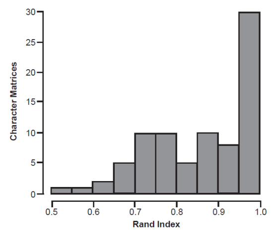
Fig. 4. Distribution of Rand indices comparing Pearson BDC and medoid partitioning for all distance matrices.
Medoid partitioning was also calculated for one fewer and one more cluster than present in the Pearson BDC partition. On average, reducing or increasing the cluster count yielded a slightly lower average silhouette width. On average, the average silhouette width for medoid partitioning into the same number of clusters detected in Pearson BDC was 0.40. For one fewer clusters, the average was 0.39, and for one more clusters, the average was 0.38. For 80% of the distance matrices, medoid partitioning into one greater or fewer clusters than the Pearson BDC cluster count yielded an average silhouette width that absolutely differed by only 0.1 or lower from the medoid partition that produced the same number of clusters as the Pearson BDC clustering. Compared directly to the Pearson BDC partition, in only 12 cases did varying the number of clusters by one produce a medoid partition that had an average silhouette width that was greater than the average silhouette width of the Pearson BDC partition. The Pearson BDC partition had an average silhouette width greater than or equal to any of the tested medoid partition average silhouette widths in 50 out of the 82 cases (61%).
Individual cluster similarity was also high, with an average Rand index between the Pearson BDC clusters and the medoid partition of 0.87 (median 0.89) when the medoid partition was calculated with the same number of Pearson BDC clusters. In 29 cases (35%), medoid partitioning produced exactly the same partition as the Pearson BDC partition. For only nine cases (11%), the Rand index was less than 0.7. The main difference between the Pearson BDC and the medoid partitioning was seen in the tendency of medoid partitioning to lump taxa together in bigger clusters. For example, where Pearson BDC produced 47 singletons for all distance matrices, medoid partitioning (at the same number of clusters observed in the Pearson BDC) produced only 34 singletons.
Fuzzy analysis on these distance matrices was more difficult than the medoid partition, because fuzzy analysis can only be done for cluster numbers up to n/2 -1, where n is the number of taxa. In cases where a few taxa are sorted into many clusters by the Pearson BDC method, fuzzy analysis could not be calculated. For the 82 distance matrices in the present study, fuzzy analysis could only be performed on 60. In 15 of those cases (25%), fuzzy analysis calculated for the same number of clusters as the Pearson BDC yielded a partition with an average silhouette width greater than the Pearson BDC partition, but 11 of those were also cases where the medoid partition for the same number of clusters as the Pearson BDC yielded an average silhouette width greater than the Pearson BDC partition. The fuzzy clustering was less similar to the Pearson BDC than the Pearson BDC clustering was to the medoid partition (average Rand index of 0.82 and 0.87 respectively). When fuzzy analysis and medoid partition were calculated at the same number of clusters as the Pearson BDC clustering, eleven distance matrices yielded exactly the same partitioning across all three methods.
The Hopkins statistics ranged from 0.63 to 0.93, with an average of 0.79 (median 0.78) (fig. 5). While the average is considerably higher than the 0.5 that indicates no clustering structure, the Hopkins statistics did not appear to correlate with consistency of different methods. Hopkins statistics were nearly identical for the 29 distance matrices where the Pearson BDC and medoid partitions were the same vs. the 53 distance matrices where they were not; both had average Hopkins statistics of 0.786. Hopkins statistics were different for the distance matrices that produced the fewest clusters in the Pearson BDC analysis. For the 58 matrices that yielded two or three Pearson BDC clusters, the average Hopkins statistic was 0.80, but for the 24 matrices that yielded four or more Pearson BDC clusters, the average Hopkins statistic was 0.73.
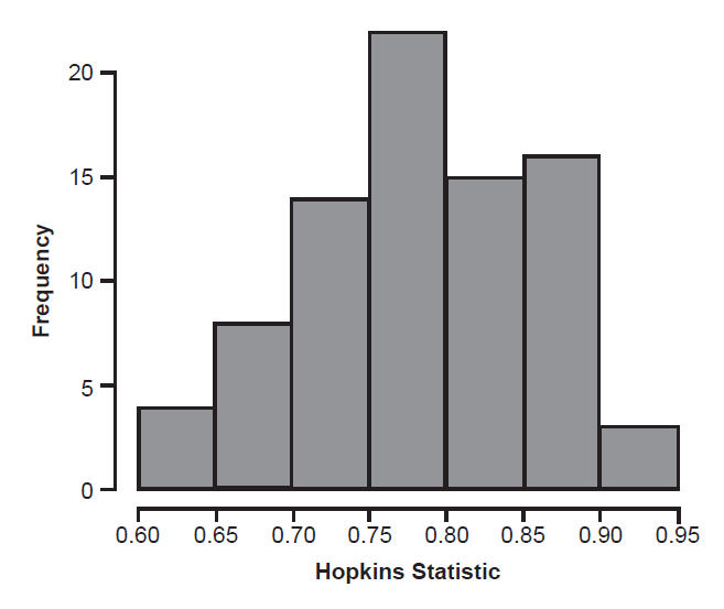
Fig. 5. Distribution of Hopkins statistic for all character matrices.
Dip test values ranged from 0.0057 to 0.12, with an average of 0.035. Unlike the Hopkins statistic, dip test values did differ when the Pearson BDC and medoid partitioning disagreed. For the 29 distance matrices where the Pearson BDC and medoid partitioning were identical, the average dip test value was 0.047, but for the 53 matrices where Pearson BDC and medoid partitioning differed, the average dip test was only 0.028. Dip test values did not differ by much when considering only the number of clusters produced by the Pearson BDC procedure. Dip test values averaged 0.034 for two or three Pearson BDC clusters vs. 0.037 for four or more clusters.
Perhaps most interestingly, dip test p-values were statistically significant for only twelve distance matrices. Those twelve had Hopkins statistics ranging from 0.68 to 0.93 with an average of 0.84. The other 70 distance matrices with nonsignificant dip tests had an average Hopkins statistic of 0.78. Three of the distance matrices with significant dip tests produced two Pearson BDC clusters, seven produced three clusters, and two produced four Pearson BDC clusters. Average silhouette widths for the Pearson BDC partitions with statistically significant dip tests ranged from 0.23 to 0.81 with an average of 0.52. For the other 70 distance matrices with nonsignificant dip tests, the average silhouette widths for the Pearson BDC partitions ranged from 0.16 to 0.7 with an average of 0.40. The twelve distance matrices with significant dip tests were also enriched in holobaramin identifications (see below). Eight of the twelve were judged to be holobaramins or possible holobaramins (67%), whereas only 56% of the distance matrices with nonsignificant dip tests were so judged.
When considered according to classification of baramins rather than mere clustering, the similarity is once again striking between the present results and those of Thompson and Wood (2018). Overall, the present baraminological classification matched that of Thompson and Wood (2018) in 54 cases (65.9%). Thompson and Wood (2018) recognized 33 holobaramins (“HB”), 24 possible holobaramins (“HB?”), and three monobaramins (“MB”). For 22 of the distance matrices, they concluded that the results were inconclusive (“Inc”). In the present study when all the results from Pearson BDC, Spearman BDC, medoid partitioning, and fuzzy analysis are considered together (see discussion in the Appendix, available online), the original conclusions are modified slightly by increasing the number of inconclusive results. Here, 29 holobaramins and 18 possible holobaramins are recognized, and 32 distance matrices are considered inconclusive. In 24 cases, the original holobaramin conclusion is confirmed. Five possible holobaramins (“HB?”) in the original study were “upgraded” to holobaramins (“HB”), but six holobaramins (“HB”) in the original study were “downgraded” to only possible holobaramins (“HB?”) in this study. Nine possible holobaramins (“HB?”) were changed to inconclusive in the present study. Three holobaramins (“HB”) from the original study were here classified as inconclusive. Three of the original inconclusive results from the original study were changed to possible holobaramins (“HB?”). The full comparison of these conclusions are shown in table 1. In the original study, 69.5% of the distance matrices yielded a conclusion of holobaramin or possible holobaramin, but in the present study, only 57.3% of the distance matrices yielded a conclusion of holobaramin or possible holobaramin. Still, nearly two thirds of conclusions (54, 65.9%)) were unchanged between the previous and present study.
| Family | Citation (see Appendix for complete citation) | Thompson and Wood (2018) | Present Study |
|---|---|---|---|
| Ornithorhynchidae | Rowe et al. 2008 | HB? | HB? |
| Paramelidae | Travouillon et al. 2014 | Inc | Inc |
| Palorchestidae | Black 2008 | HB | HB |
| Thylacoleonidae | Gillespie 2007 | HB? | Inc |
| Hypsiprymnodontidae | Bates et al. 2014 | HB | HB |
| Macropodidae | Prideaux and Tedford 2012 | HB? | Inc |
| Macropodidae | Kear et al. 2007 | HB | HB |
| Pseudocheirinae | Springer 1993 | HB | HB |
| Phascolarctidae | Black et al. 2012 | HB | HB |
| Didelphidae | Voss and Jansa 2009 | HB? | Inc |
| Caenolestidae | Ojala-Barbour et al. 2013 | MB | MB |
| Hathliacynidae | Forasiepi et al. 2006 | HB? | MB |
| Dasypodidae | Herrera et al. 2017 | HB | HB? |
| Glyptodontidae | Zurita et al. 2013 | HB | HB |
| Myrmecophagidae | Gaudin and Branham 1998 | HB? | HB |
| Pseudorhyncocyonidae | Hooker 2013 | HB? | HB? |
| Ochotonidae | Fostowicz-Frelik et al. 2010 | Inc | Inc |
| Leporidae | Fostowicz-Frelik 2013 | Inc | Inc |
| Aplodontidae | Hopkins 2008 | Inc | Inc |
| Castoridae | Rybczynski 2007 | HB | HB? |
| Cricetidae | Maridet and Ni 2013 | Inc | Inc |
| Anomaluridae | Sallam et al. 2010 | HB | HB |
| Caviidae | Pérez and Vucetich 2011 | HB? | Inc |
| Octodontidae | Verzi et al. 2013 | Inc | Inc |
| Echimyidae | Carvallo and Salles 2004 | Inc | Inc |
| Palaeoryctidae | Rankin and Holroyd 2014 | Inc | Inc |
| Manidae | Kondrashov and Agadjanian 2012 | HB | HB |
| Hyaenodontidae | Polly 1996 | Inc | HB? |
| Felidae | Holliday 2007 | HB | HB |
| Machairodontinae | Christiansen 2013 | HB | Inc |
| Barbourofelinae | Morlo et al. 2004 | Inc | HB? |
| Ursidae | Abella 2012 | HB? | Inc |
| Otariidae | Churchill et al. 2014 | HB | Inc |
| Odobenidae | Boessenecker and Churchill 2013 | HB? | HB? |
| Mustelidae | Prevosti and Ferrero 2008 | HB | HB? |
| Mephitinae | Wang et al. 2014 | HB | Inc |
| Procyonidae | Ahrens 2012 | Inc | Inc |
| Chrysochloridae | Asher et al. 2010 | HB | HB |
| Erinaceidae | He et al. 2012 | HB | HB |
| Talpidae | Sánchez-Villagra et al. 2006 | HB | HB |
| Nyctitheriidae | Manz and Bloch 2015 | HB? | Inc |
| Soricidae | Hugueney and Maridet 2011 | HB? | HB |
| Rhinolophidae | Hand and Kirsch 2003 | HB? | Inc |
| Mormoopidae | Simmons and Conway 2001 | MB | Inc |
| Phyllostomidae | Wetterer et al. 2000 | Inc | Inc |
| Picrodontidae | Burger 2013 | HB | HB |
| Plesiadapidae | Burger 2013 | HB | HB |
| Lemuridae | Herrera and Dávalos 2016 | HB | HB |
| Lepilemuridae | Herrera and Dávalos 2016 | HB | HB |
| Loridae | Masters et al. 2005 | Inc | Inc |
| Carpolestidae | Bloch et al. 2001 | HB? | HB? |
| Omomyidae | Ni et al. 2004 | HB | HB? |
| Cebidae | Garbino 2015 | HB? | HB? |
| Cebidae | Schrago et al. 2013 | Inc | HB? |
| Orycteropodidae | Lehmann 2009 | Inc | Inc |
| Louisinidae | Hooker and Russell 2012 | Inc | Inc |
| Hyopsodontidae | Williamson and Weil 2011 | Inc | Inc |
| Didolodontidae | Gelfo and Siegé 2011 | HB? | HB? |
| Suidae | Orliac et al. 2010 | HB | HB? |
| Hippopotamidae | Boisserie et al. 2010 | HB? | HB? |
| Anthracotheriidae | Rincon et al. 2013 | Inc | Inc |
| Camelidae | Scherer 2013 | HB? | Inc |
| Moschidae | Sanchez et al. 2010 | MB | MB |
| Cervidae | Lister et al. 2005 | Inc | Inc |
| Notohippidae | Cerdeño and Vera 2010 | Inc | Inc |
| Leontiniidae | Schockey et al. 2012 | HB | HB |
| Toxodontidae | Forasiepi et al. 2015 | HB | HB |
| Interatheriidae | Reguero et al. 2003 | Inc | Inc |
| Interatheriidae | Hitz et al. 2006 | HB | HB |
| Hegetotheriidae | Billet et al. 2009 | HB | HB |
| Astrapotheriidae | Vallejo-Pareja et al. 2015 | HB | HB |
| Carodniidae | Antoine et al. 2015 | HB? | HB |
| Palaeotheriidae | Danilo et al. 2013 | HB | HB? |
| Brontotheriidae | Mihlbachler 2008 | HB? | Inc |
| Chalicotheriidae | Bai et al. 2010 | HB? | HB? |
| Rhinocerotidae | Becker et al. 2013 | Inc | Inc |
| Lophiodontidae | Robinet et al. 2015 | HB | HB |
| Sirenia | Sorbi 2008 | HB | HB |
| Desmostylidae | Beatty 2009 | HB? | HB? |
| Procaviidae | Seiffert et al. 2012 | HB | HB |
| Gompotheriidae | Cozzuol et al. 2012 | HB? | HB |
| Elephantidae | Ferretti and Debruyne 2010 | HB? | HB |
We can compare the 47 distance matrices classified as “HB” or “HB?” to the 32 distance matrices classified as inconclusive (“Inc”) in the present study. We find that the dip test varies substantially between the two groups, with an average of 0.039 for the HB/HB? matrices and 0.026 for the inconclusive matrices. Curiously, the Hopkins statistic was nearly the same (0.79 average for HB/HB? and 0.8 average for inconclusive matrices). The average silhouette widths of the Pearson BDC clustering tend to be higher on average for the HB/HB? matrices than the inconclusive matrices (averages 0.44 vs. 0.38). On average, HB/HB? distance matrices came from character sets with a higher number of characters (mean 76.6) and a lower number of OTUs (mean 20.6) than the inconclusive distance matrices (means 63.8 and 28.3 respectively).
Discussion: Expanding the Toolkit of Baraminology Techniques
According to Reeves (2021a, b), BDC is formally invalid, and its utility as a heuristic is unknowable. To assess whether the BDC heuristic is useful, I examined a previously published set of BDC analyses to determine the consistency of Pearson BDC with published phylogenies, BDC calculated with Spearman correlations, medoid partitioning, and fuzzy analysis. I found a good agreement between all methods tested. Compared to published phylogenies, Pearson BDC clusters were monophyletic in nearly 70% of cases. Compared to Spearman BDC, the Pearson BDC clusters matched exactly in 31 of 82 cases (37.8%), and the similarity between all Spearman and Pearson BDC clusters was high, with a Rand index of 0.9. When calculated for the same number of clusters as the Pearson BDC, the medoid partitioning produced identical clusters to the Pearson BDC in 29 cases (35.4%) and the average Rand index was 0.87, once again revealing a very close match between most Pearson BDC and medoid partitions. When calculated for the same number of clusters as the Pearson BDC, fuzzy analysis produced the same clusters as the BDC partition in only 15 (25%) out of the 60 cases where fuzzy analysis could be applied, but once again the average Rand index of 0.82 was very high.
We can also assess cluster agreement using the average silhouette width, which evaluates clusters independently of the method by which they are generated. Of the four partitioning methods evaluated here, Spearman BDC produces the highest average silhouette widths (mean 0.42), and medoid partitioning produces the lowest (mean 0.40), but the difference is slight. Pearson BDC performs nearly as well as the Spearman BDC (mean 0.416 vs 0.417) and fuzzy analysis (mean 0.416 vs. 0.414).
Considering these results, we can see that Pearson BDC, the method used in dozens of published baraminology articles, performs at least as well as if not better than medoid partitioning or fuzzy analysis, which were recommended by Reeves to replace BDC. Therefore, rather than merely criticizing BDC, future research ought to determine why Pearson BDC performs so well, given that it violates certain methodological assumptions. As things stand, it would seem that past results need not be questioned or discarded only because they are based in part or in whole on Pearson BDC. Likewise, my previous recommendation that Pearson BDC be deprecated in favor of Spearman BDC (Wood 2020) was premature and unwarranted.
Just as important as the general reliability of Pearson BDC is the strong disagreements between the methods. In this sample of 82 studies, I found the baraminological conclusions changed from 57 to 47 holobaramins or possible holobaramins (decrease of 17.5%) and from 22 to 32 inconclusive results (increase of 45.5%). Thus, while the results overall still favor recognizing holobaramins by statistical baraminology, consideration of additional clustering techniques unsurprisingly increases the uncertainty of some results.
There were twelve (14.6%) distance matrices where the new evidence from the Spearman BDC, medoid partitioning, and fuzzy analysis warranted changing the original researchers’ conclusion from holobaramin or possible holobaramin to inconclusive. In the case of the Didelphidae from a character set used by Voss and Jansa (2009), there was very little agreement between the different clustering methods, hence justifying viewing the original results with much greater uncertainty (Appendix, 56-61). In the case of the Mephitidae using a character set from Wang, Carranza-Castañeda, and Aranda-Gómez (2014), the Pearson BDC produced three clusters with an average silhouette width of 0.34, but the medoid partition at three clusters had a considerably better average silhouette width of 0.43. The fuzzy analysis at three clusters differed from the medoid partition by only a single taxon but still had an average silhouette width of 0.43 (Appendix, 211-216). Since the cluster analysis methods produced better clustering than the Pearson BDC, we are justified in questioning the original conclusions.
As noted, substitution of Spearman correlations for Pearson results in an increase in “significant” positive correlation and a decrease in “significant” negative correlation. This is to be expected, since Spearman uses ranks and therefore can detect nonlinear correlations. As a result, Spearman-based BDC produces fewer clusters than Pearson BDC in 48 of 82 cases (58.5%). In only three cases did Spearman-based BDC produce more clusters than the Pearson BDC. Additionally, since discontinuity is inferred from patterns of “significant,” negative BDC, Spearman would be ill-suited for inferring discontinuity in future studies due to the dearth of negative BDC.
Because medoid partitioning works by minimizing the distance between a cluster’s centrally-located medoid and all other members of that cluster, medoid partitioning works best with globular or spherical clusters. Since we have no reason to expect that taxa will be distributed in a globular fashion (whether they belong to the same baramin or not), the utility of medoid partitioning may be limited. For example, if future studies apply medoid partitioning to an elongate cluster of points (for example, Cavanaugh, Wood, and Wise 2003), we would expect the mostly continuous linear form to be divided into multiple clusters.
Of all the methods presented here, fuzzy analysis produced the most divergent partitions. Compared to medoid partitioning and Pearson BDC with the same number of clusters, fuzzy analysis produced a partition identical to Pearson BDC only 15 times and identical to medoid partitioning only 19 times. In contrast, Pearson BDC and medoid partitioning produced the same clusters 26 times. Thus, in future work, researchers should consider using and interpreting fuzzy analysis with care, recognizing that differences observed using fuzzy analysis may be methodological artifacts.
Most interesting of all, the Hopkins statistic and dip test did not strongly support the presence of clusterability in the distance matrices. The present implementation of the Hopkins statistic does not follow the recommendation of sampling only 5–10% of the taxa (since there are so few taxa), and therefore the statistical significance of the statistic cannot be estimated from a beta distribution. As noted above, the Hopkins statistic ranges from 0.5 to 1, with higher numbers indicating more deviation from a random distribution of points. Since the average Hopkins statistic was 0.79, we may infer that the average distance matrix here does contain clusters. This would be consistent with the observation that none of the distance matrices yielded only a single Pearson BDC cluster, even though a single cluster is a possible outcome. Also interesting is the observation that the average Hopkins statistic was higher for distance matrices with fewer clusters. Since the Hopkins statistic compares nearest neighbor distances between real points and a set of points drawn from a uniform distribution, concentrating real points into a small number of clusters ought to produce a higher Hopkins statistic than spreading the same number of points out in a greater number of clusters. In future research, it might be possible to estimate the significance of any Hopkins statistic empirically through Monte Carlo simulations.
The fact that the dip test revealed so few instances of significant clustering is not surprising, given the type of distance matrices in the present study. In previous simulation research, the dip test performed worst when presented with a single cluster and multiple outliers (Adolffson, Ackerman, and Brownstein 2019), even though it was generally a very reliable clusterability statistic. Thompson and Wood (2018) selected their set of mammal character sets precisely on that characteristic: a good sample of ingroup taxa with a smaller sample of outgroup taxa. Add to that the small number of taxa (average of 23), and we might expect very few of these distance matrices to exhibit clusterability as measured by the dip test.
Indeed, we can evaluate this with very simple simulations (fig. 5). For a two dimensional cluster of twenty points with x and y coordinates randomly drawn from a normal distribution (mean 0, standard deviation 1), we can add one additional point at coordinates x = 5, y = 5, which represents the outlier or singleton cluster. Visually, this 2D array of points appears to be a cluster with an individual point at noticeable distance (fig. 6), but the Euclidean distances between all 21 points appears to be a unimodal distribution. The dip test bears this out, revealing that the distance distribution is not clusterable. In a sample of 100 such simulations, only once did the dip test produce a statistically significant result. Thus, the dip test appears to have limited applicability in most baraminological studies.
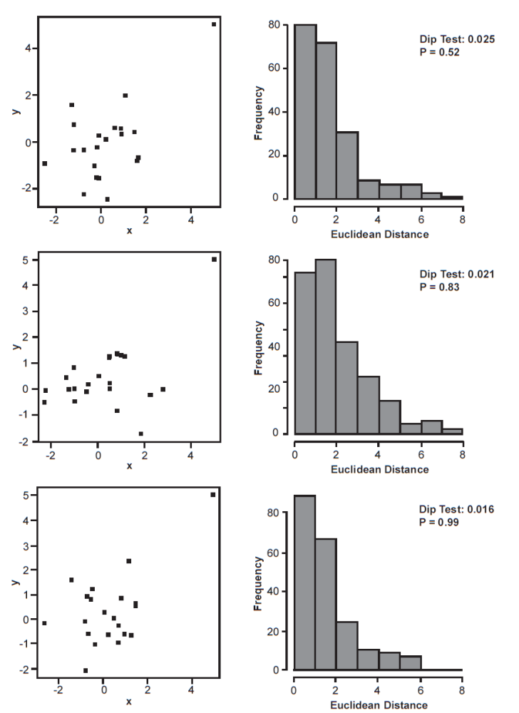
Fig. 6. Sample of three simulations showing a normally distributed, two-dimensional cluster, wherein 20 x and y coordinates are drawn randomly from a normal distribution with mean of 0 and standard deviation of 1. The outgroup or singleton taxon is shown at coordinates x = 5, y = 5. For each set of 21 points, the distribution of Euclidean distances between the points are also shown, along with the dip test statistic and p-value.
Based on these results, we may consider three issues for future research. First, baraminology studies absolutely must consider more than one method of clustering. The BDC method (Pearson or Spearman) has the advantage of indicating a specific number of clusters present, while medoid partitioning and fuzzy analysis must be used to confirm these results, with the recognition that fuzzy clustering often disagrees with other methods. Second, the use of clusterability statistics warrants further research before overly relying on these to indicate the presence of a possible holobaramin. Third, to test the discontinuity hypothesis, statistical baraminology methods must be applied at multiple taxonomic levels.
Additional questions raised by Reeves remain unanswered in this present study. Among them are the efficacy of the bootstrap when applied to the new methodology. Since bootstrapping has been shown to be a valuable assessment of the robustness of phylogenetic and baraminology hypotheses, its use in cluster analysis ought to be explored as well.
Reeves also reveals an aversion to conclusions about the human holobaramin, which despite his concern with the technical legitimacy of statistical baraminology, he never quantifies. Nonetheless, these new methods ought to be applied to hominin fossil character matrices to determine if any previous conclusions should be modified in light of these new techniques. This work is presently ongoing, and I anticipate publication of the preliminary results within a year’s time.
In conclusion, while the Pearson BDC as a heuristic is not as dubious as Reeves implies, the addition of cluster analysis techniques unquestionably strengthens the statistical baraminology toolkit. While some of Reeves’s claims were faulty, we definitely owe him a debt of gratitude for pushing statistical baraminology into new methodological territory.
References
Adolfsson, Andreas, Margareta Ackerman, and Naomi C. Brownstein. 2019. “To Cluster, or Not to Cluster: An Analysis of Clusterability Methods.” Pattern Recognition 88 (April): 13–26.
Bermúdez-de-Castro, José-María, María Martinón-Torres, Laura Martín-Francés, Mario Modesto-Mata, Marina Martínez-de-Pinillos, Cecilia García, and Eudald Carbonell. 2017. “Homo antecessor: The State of the Art Eighteen Years Later.” Quaternary International 433A (17 March): 22–31.
Cavanaugh, David P., and Richard V. Sternberg. 2002. “Analysis of Morphological Constraints Using ANOPA, a Pattern Recognition and Multivariate Statistical Method: A Case Study Involving Centrarchid Fishes.” Journal of Biological Systems 12, no. 2 (November): 137–167.
Cavanaugh, David P., and Todd Charles Wood. 2002. “A Baraminological Analysis of the Tribe Heliantheae sensu lato (Asteraceae) Using Analysis of Pattern (ANOPA).” Occasional Papers of the BSG 1 (June 17): 1–11.
Cavanaugh, David P., Todd Charles Wood, and Kurt P. Wise. 2003. “Fossil Equidae: A Monobaraminic, Stratomorphic Series.” In Proceedings of the Fifth International Conference on Creationism. Edited by Robert L. Ivey, Jr., 143–153. Pittsburgh, Pennsylvania: Creation Science Fellowship.
Chapman, Geoff. 1991. “Horse Non-sense!” Creation Ex Nihilo 14, no. 1 (December): 50.
Dembo, Mana, Davorka Radovčić, Heather M. Garvin, Myra F. Laird, Lauren Schroeder, Jill E. Scott, Juliet Brophy, Rebecca R. Ackermann, Chares M. Musiba, Darryl J. de Ruiter, Arne Ø. Mooers, and Mark Collard. 2016. “The Evolutionary Relationships and Age of Homo naledi: An Assessment Using Dated Bayesian Phylogenetic Methods.” Journal of Human Evolution 97 (August): 17–26.
DuBois, Paul. 1988. “Creationist Evaluation of Australopithecus afarensis.” Creation Research Society Quarterly 25, no. 2 (September): 65–69.
Evander, R. L. 1989. “Phylogeny of the Family Equidae.” In The Evolution of the Perissodactyls. Edited by D. R. Prothero, and R. M. Schoch, 109–127. New York: Oxford University Press.
Garner, Paul A., Todd C. Wood, and Marcus Ross. 2013. “Baraminological Analysis of Jurassic and Cretaceous Avialae.” In Proceedings of the Seventh International Conference on Creationism. Edited by Mark Horstemeyer, Article 16. Pittsburgh, Pennsylvania: Creation Science Fellowship.
Haile-Selassie, Yohannes, Stephanie M. Melillo, Antonino Vazzana, Stefano Benazzi, and Timothy M. Ryan. 2019. “A 3.8-million-year-old Hominin Cranium From Woranso-Mille, Ethiopia.” Nature 573, no. 7773 (12 September): 214–219.
Hartigan, J. A., and P. M. Hartigan. 1985. “The Dip Test of Unimodality.” Annals of Statistics 13, no. 1 (March): 70–84.
Heintzman, Peter D., Grant D. Zazula, James A. Cahill, Alberto V. Reyes, Ross D. E. MacPhee, and Beth Shapiro. 2015. “Genomic Data From Extinct North American Camelops Revise Camel Evolutionary History.” Molecular Biology and Evolution 32, no. 9 (September): 2433–2440.
Hopkins, Brian, and J. G. Skellam. 1954. “A New Method For Determining the Type of Distribution of Plant Individuals.” Annals of Botany 18, no. 79 (April): 213–227.
Hubert, Lawrence and Phips Arabie. 1985. “Comparing Partitions.” Journal of Classification 2 (December): 193– 218.
Isaac, Randy. 2007. “Assessing the RATE Project.” Perspectives on Science and the Christian Faith 59 (June): 143–146.
Leakey, Meave G., Craig S. Feibel, Ian McDougall, and Alan Walker. 1995. “New Four-Million-Year-Old Hominid Species From Kanapoi and Allia Bay, Kenya.” Nature 376, no. 6541 (17 August): 565–571.
Marsh, Frank Lewis. 1944. Evolution, Creation, and Science. Washington, DC: Review and Herald Publishing Association.
McLain, Matthew, Matt Petrone, and Matthew Speights. 2018. “Feathered Dinosaurs Reconsidered: New Insights From Baraminology and Ethnotaxonomy.” In Proceedings of the Eighth International Conference on Creationism. Edited by J. H. Whitmore, 472–515. Pittsburgh, Pennsylvania: Creation Science Fellowship.
Menton, David N. 2010. “Baraminological Analysis Places Homo habilis, Homo rudolfensis, and Australopithecus sediba in the Human Holobaramin: Discussion.” Answers Research Journal 3 (25 August): 153–155. https://assets.answersresearchjournal.org/doc/v3/hominid-baraminology-discussion.pdf.
Molén, Mats. 2009. “The Evolution Of the Horse.” Journal of Creation 23, no. 2 (August): 59–63.
Rand, William M. 1971. “Objective Criteria For the Evaluation of Clustering Methods.” Journal of the American Statistical Association 66, no. 336 (5 April): 846–850.
Reeves, Colin R. 2021a. “A Critical Evaluation of Statistical Baraminology: Part 1—Statistical Principles.” Answers Research Journal 14: 261–269.
Reeves, Colin R. 2021b. “A Critical Evaluation of Statistical Baraminology: Part 2—Alternatives and Conceptual and Practical Issues.” Answers Research Journal 14: 271–282.
Robinson, D. Ashley, and David P. Cavanaugh. 1998a. “A Quantitative Approach to Baraminology With Examples From the Catarrhine Primates.” Creation Research Society Quarterly 34, no. 4 (March): 196–208.
Robinson, D. Ashley, and David P. Cavanaugh. 1998b. “Evidence for a Holobaraminic Origin Of the Cats.” Creation Research Society Quarterly 35, no. 1 (June): 2–14.
Senter, Phil. 2010. “Using Creation Science to Demonstrate Evolution: Application of a Creationist Method For Visualizing Gaps in the Fossil Record to a Phylogenetic Study of Coelurosaurian Dinosaurs.” Journal of Evolutionary Biology 23, no. 8 (August): 1732–1743.
Thompson, C., and Todd Charles Wood. 2018. “A Survey of Cenozoic Mammal Baramins.” In Proceedings of the Eighth International Conference on Creationism. Edited by J. H. Whitmore, 217–221. Pittsburgh, Pennsylvania: Creation Science Fellowship.
Travouillon, K. J., S. J. Hand, M. Archer, and K. H. Black. 2014. “Earliest Modern Bandicoot and Bilby (Marsupialia, Peramelidae, and Thylacomyidae) From the Miocene of the Riversleigh World Heritage Area, Northwestern Queensland, Australia.” Journal of Vertebrate Paleontology 34, no. 2 (March): 375–382.
Voss, Robert S. and Sharon A. Jansa. 2009. “Phylogenetic Relationships and Classification of Didelphid Marsupials, an Extant Radiation of New World Metatherian Mammals.” Bulletin of the American Museum of Natural History 322: 1–177.
Wang, Xiaoming, Óscar Carranza-Castañeda, and José Jorge Aranda-Gómez. 2014. “A Transitional Skunk, Buisnictis metabatos sp. nov. (Mephitidae, Carnivora), From Baja California Sur and the Role of Southern Refugia in Skunk Evolution.” Journal of Systematic Palaeontology 12, no. 3 (May): 291–302.
Ward, Carol, Meave Leakey, and Alan Walker. 1999. “The New Hominid Species Australopithecus anamensis.” Evolutionary Anthropology 7, no. 6 (May): 197–205.
Ward, C. V., J. M. Plavcan, and F. K. Manthi. 2020. “New Fossils of Australopithecus annamensis From Kanapoi, West Turkana, Kenya (2012-2015).” Journal of Human Evolution, 140 (March). DOI 10.1016/j.jhevol.2017.07.008.
Wieland, Carl. 1990. “Fuzzy Feathers and Walking Whales.” Creation Ex Nihilo 13, no. 1 (December): 48–50.
Williams, Alex. 2004. “Baraminology, Biology and the Bible: A Review of Understanding the Pattern of Life: Origins and Organization of the Species by Todd Charles Wood and Megan J. Murray.” TJ 18, no. 2 (August): 53–54.
Wolfrom, Glen W. 2003. “A Family Affair: Close Encounters with the Camel Kind.” Creation Matters 8, no. 1 (Jan/Feb): 4–5.
Wood, Todd Charles. 2005a. “Visualizing Baraminic Distances Using Classical Multidimensional Scaling.” Origins 57 (January 1): 9–29.
Wood, Todd Charles. 2005b. “A Creationist Review and Preliminary Analysis Of the History, Geology, Climate, and Biology of the Galápagos Islands.” CORE Issues in Creation 1 (June 15): 1–241.
Wood, Todd Charles. 2008a. “Baraminic Distance, Bootstraps, and BDISTMDS.” Occasional Papers of the BSG 12 (October 3): 1–17.
Wood, Todd Charles. 2008b. “Animal and Plant Baramins.” CORE Issues in Creation 3 (November 7): 1–258.
Wood, Todd C. 2011a. “Baraminology, the Image of God, and Australopithecus sediba.” Journal of Creation Theology and Science Series B: Life Sciences 1, no. 7 (July 8): 6–14.
Wood, Todd Charles. 2011b. “Using Creation Science to Demonstrate Evolution? Senter’s Strategy Revisited.” Journal of Evolutionary Biology 24, no. 4 (April): 914–918.
Wood, Todd C. 2013. “Australopithecus sediba, Statistical Baraminology, and Challenges to Identifying the Human Holobaramin.” In Proceedings of the Seventh International Conference on Creationism. Edited by Mark Horstemeyer, Article 16. Pittsburgh, Pennsylvania: Creation Science Fellowship.
Wood, Todd Charles. 2016. “Taxon Sample Size in Hominin Baraminology: A Response to O’Micks.” Answers Research Journal 9 (December 28): 369–372. https://assets.answersresearchjournal.org/doc/v9/taxon_hominin_baraminology_response.pdf.
Wood, Todd Charles. 2017. “Identifying Humans in the Fossil Record: A Further Response to O’Micks.” Answers Research Journal 10 (Feburary 15): 57–62. https://assets.answersresearchjournal.org/doc/v10/homo_naledi_response.pdf.
Wood, Todd C. 2020. “Expanding the Toolkit of Statistical Baraminology with BARCLAY: Baraminology and Cluster Analysis.” Journal of Creation Theology and Science Series B: Life Sciences 10: 7.
Wood, Todd Charles, and Megan J. Murray. 2003. Understanding the Pattern of Life: Origins and Organization of the Species. Nashville, Tennessee: Broadman and Holman.
Wood, Todd Charles, Kurt P. Wise, Roger Sanders, and Neal Doran. 2003. “A Refined Baramin Concept.” Occasional Papers of the BSG 3 (July 25): 1–14.
Supplementary Material
The Appendix is available as a single pdf file at https://assets.answersresearchjournal.org/doc/articles/arj/v14/reeves-response-appendix.pdf.


