The Case for Cosmological Redshifts

Introduction

Edwin Hubble (1929) is credited with the discovery of the expansion of the universe. Technically, Hubble found the Hubble relation, a linear relationship between galaxy redshift and distance (see Fig. 1 for a reproduction of Hubble’s original 1929 plot). Note that the horizontal axis is in terms of parsecs (pc), the preferred unit of distance outside the solar system. The vertical axis is in terms of velocity (though Hubble omitted the “per second” in the units). While one can express redshift in velocity, it is more common today to use the unitless quantity z = Δλ/λ, where λ is the rest wavelength of a spectral line and Δλ is its shift in wavelength.1 When z is positive, an object’s distance is increasing, and its wavelength is shifted toward longer wavelengths, corresponding to red in the visible spectrum. However, when z is negative, an object’s distance is decreasing, and the shift in its spectrum is toward shorter wavelengths, corresponding to blue in the visible spectrum. Hence, positive z is called a redshift, while a negative z is called a blueshift.

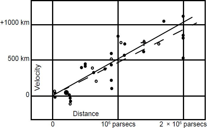
Fig. 1. Hubble’s original plot of the Hubble relation. The dots represent measurements of redshifts and distances of 24 galaxies. The solid line is the linear fit to those 24 points. The circles represent binning of those 24 galaxies, with the dashed line being the fit to those points. The cross represents the mean velocity and distance of 22 galaxies for which individual distance measurements were not possible.

Redshifts of extragalactic objects are the sum of two distinct effects, one local, and one global. Gravity of local objects accelerate galaxies so that they move with respect to space. For simplicity, we can call this Doppler motion, because the component of this motion in our line of sight is measured via the Doppler effect. The exact (special relativistic) equation relating velocity to redshift for Doppler motion is

However, the exact equation is of little relevance to our discussion, because the velocities of stars and large assemblages of stars, such as galaxies, never approach c.2 For small z, a Taylor series expansion reduces this to the simple approximation,

Doppler motions of galaxies typically have magnitude of hundreds to a little more than a thousand km/s, depending upon the amount of local matter present.3 They cluster around zero value, with half of Doppler motions being positive and half being negative.

In the context of cosmology, the global effect due to the expansion of the universe is far more important than the Doppler component. When general relativity is applied to the universe, the most general solution is that the universe is either expanding or contracting. It is a matter of observation to determine which is the correct solution for the universe. The prediction is that if the universe is expanding, then redshift will increase with increasing distance. On the other hand, if the universe is contracting, redshift will decrease with increasing distance. Since the Hubble relation confirms the former, it appears that the universe is expanding. The redshift due to expansion may be given simply as:

where a₀ is current scale factor of the universe, and a is the scale factor at the time when light we are now receiving from distant objects was emitted. The scale factor is a function of time. Since this redshift is due to an effect of cosmology, we say that redshifts of this nature are cosmological. Unlike Doppler motion, cosmic expansion always results in positive redshift. Furthermore, cosmic redshift increases with increasing distance. However, observationally it is impossible to distinguish between Doppler motion and cosmological redshift. Therefore, it is not possible to determine how much of an extragalactic object’s redshift is due to cosmic expansion and how much is due to Doppler motion. Undoubtedly, the redshift of nearby galaxies is dominated by Doppler motion, while the redshifts of distant galaxies are dominated by cosmic expansion. At sufficient distance, Doppler motion is so modest as compared to cosmic expansion that it is negligible.

Initially, astronomers and cosmologists interpreted universal expansion as Doppler motion. However, this is incorrect. Unfortunately, many treatments of the Hubble relation fail to make this distinction. Adding to the confusion, for modest redshifts (z << 0), there is no appreciable difference between the correct treatment and the incorrect treatment. In the creation literature of the past half-century, many discussions of cosmology continued to confuse cosmic expansion with Doppler motion. This is regrettable, and we ought to strive to eliminate this practice.

Immediately after Hubble’s discovery, there was debate over what the redshifts of extragalactic objects meant. As defined above, cosmological redshifts mean that the universe is expanding so that redshifts reflect distance. However, some questioned whether the universe was expanding while simultaneously accepting the Hubble relation so that redshifts indicate distance. Most notable is the “tired light” proposal of Zwicky (1929). According to this hypothesis, an unidentified agent redshifted light as it traveled through space. The greater the distance, the greater the redshift, so the Hubble relation is true, but without an expanding universe. This discussion gradually waned, only to be reignited in the 1960s with the discovery of quasars. Since then, the debate has waned considerably once again.

However, within the recent creation community there remains considerable doubt about redshifts being cosmological (for example, Ettari 1989; Hartnett 2004a). Among recent creationists, there appears to be confusion about three related questions:

1. Is the universe expanding?
2. Do galaxy redshifts indicate distance?
3. Do quasar redshifts indicate distance?

Most astronomers would answer all three questions in the affirmative. However, many recent creationists would answer one or more of these questions in the negative. Let me address each of these questions, starting with the first one. Opposition to an expanding universe appears to be motivated by opposition to the big bang model. Obviously, if the universe is not expanding, then the big bang could not have happened. However, the big bang model is not the only possible cosmology/cosmogony based upon an expanding universe. For instance, the eternal steady state model also was based upon an expanding universe. What if the universe is expanding? If so, then the rejection of that concept would make it impossible to develop a biblical cosmological model. The expanding universe was a prediction of general relativity, one of the most tested theories of physics. I find it interesting that some recent creationists who appear to accept general relativity reject this prediction of that theory.

As for the second question, the Hubble relation appears to show that the redshift and distance are related. In the intervening nine decades since Hubble’s original publication, the Hubble relation has been confirmed repeatedly with an incredible amount of diverse data. The Hubble constant, H₀, is the slope of the Hubble relation. If the Hubble relation holds for other extragalactic objects (generally other galaxies), then we can use H₀ in the Hubble relation to find distances of those extragalactic objects. This is a matter of pure observational science, so it is difficult to understand why anyone would question this.

The third question is to ask whether the Hubble relation applies to quasars as well as galaxies. This issue arose in the late 1960s as some astronomers committed to the steady state model realized that the lack of local quasars disproved the steady state model. Many recent creationists have triumphed the work of these doubters (mostly Halton Arp) without realizing the agenda of these people. Furthermore, many recent creationists who reference Arp’s work appear to think Arp doubted the expansion of the universe and that most extragalactic redshifts were cosmological. To the contrary, Arp believed the universe to be expanding; otherwise, his preferred model, the steady state, would not work. And Arp accepted that most galaxy redshifts were cosmological. Rather, Arp opposed what he thought was a slavish devotion to cosmological redshifts. He thought that astronomers erred when they assumed that quasar redshifts were cosmological, because he argued that quasars are much closer than their redshifts would indicate.

It is my purpose here to address these doubts among recent creationists. I encourage recent creationists to answer the second and third questions in the affirmative, for there are good observational reasons to do so. These observations are relatively free of assumptions about the past. While the first question is more theoretical and could be subject to philosophical assumptions, I encourage recent creationists to answer that question affirmatively, because it is the best interpretation of the data.

What is the Value of H₀?

Not only is the Hubble relation useful for finding extragalactic distances, it is of immense importance in cosmology. The most straightforward interpretation of the Hubble relation is that the universe is expanding. If this is true, then H₀ measures the expansion rate. Either way, knowing the value of H₀ is vitally important. Hubble initially determined H₀ to be 500 km/s/Mpc, but it was clear that this was at best a preliminary result. Over the next three decades, the value of H₀ steadily decreased until by the 1960s its standard value was 55 km/s/Mpc, where it remained for another three decades. In the early 1990s, the Hubble constant underwent major reevaluation, and, for the first time, its value was revised upward. Today, the best estimate of H₀ is about 70 km/s/Mpc. (The two current major determinations of The Hubble constant are 73 ± 2 km/s/Mpc from Cepheid variables and type Ia supernovae, and 66.9 ± 0.6 km/s/Mpc inferred from the cosmic microwave background CMB.4 Note they do not overlap, and this is now recognized as a major problem in astronomy and cosmology. Also note that the first value is from direct observation, while the second is highly model dependent.)

Why the huge range? Redshift data are relatively unambiguous. Redshift measurement requires spectroscopy, which is an inefficient use of light coming from what are already very dim sources in this case. This requires large telescope aperture and sensitive detectors. However, once redshifts are measured, there is not much disagreement as to their values. However, distance is another matter. See Faulkner (2013) for a discussion of astronomical distance determination methods. Trigonometric parallax, the only direct method of measuring stellar distances, is far too limited in range to be of use in determining extragalactic distances. Therefore, astronomers use standard candles as indirect methods to measure the distances of galaxies. The best known standard candle is Cepheid variables. Many of the early decreases in the value of the Hubble constant were due to improved understanding in these standard candles. For instance, one of the major downward revisions of H₀ was in the 1950s, when astronomers realized that there were two types of Cepheid variables. However, even with today’s best technology, most standard candles cannot be seen beyond about 15 Mpc, defining the upper limit for their use.

This brings up the most challenging problem in measuring H₀. If the universe is expanding, then the observed redshift of a galaxy is the sum of its cosmological redshift, or Hubble flow, caused by expansion of the universe, and the galaxy’s Doppler motion due to local effects of gravity. While the Hubble flow component of redshift always is positive, the Doppler component can be either positive or negative. Furthermore, while Hubble flow increases linearly with distance, Doppler motion ought to fluctuate positively and negatively around an average value of zero for any given region of space. The result is that the redshifts of nearby galaxies are dominated by Doppler motion, while the redshifts of distant galaxies are dominated by Hubble flow. Observationally, Hubble flow and Doppler motion are indistinguishable, so there is no way to determine what portion of a galaxy’s redshift is due to Hubble flow and what portion is due to Doppler motion.

The best example of this problem is the Andromeda Galaxy (M31), illustrated in Fig. 2. At nearly 0.8 Mpc, M31 is the closest galaxy of any size (Like the Milky Way, it is a large spiral). Assuming H₀ is 70 km/s/Mpc, we would expect the Hubble flow of M31 to be about 50 km/s, but we also would expect the magnitude of M31’s Doppler motions to exceed this. The measured redshift of M31 is −300 km/s (z = −0.001), the negative sign indicating that its motion is toward us and thus is a blueshift. This is not surprising, because astronomers think M31 and the Milky Way Galaxy (our galaxy) orbit one another (possibly merging in the future?). M31 is the only galaxy of any size with an observed blueshift (M33, another nearby spiral galaxy, also has a slight blueshift, but it is smaller than the Milky Way and M31). How do we know what the typical Doppler motion of galaxies is? Most galaxies are in large clusters of galaxies. The Milky Way and M31 are unusual in this respect, because they are not part of a large cluster of galaxies. Instead, these two large galaxies, along with M33, dominate the Local Group, consisting of these three galaxies and more than 50 much smaller galaxies.

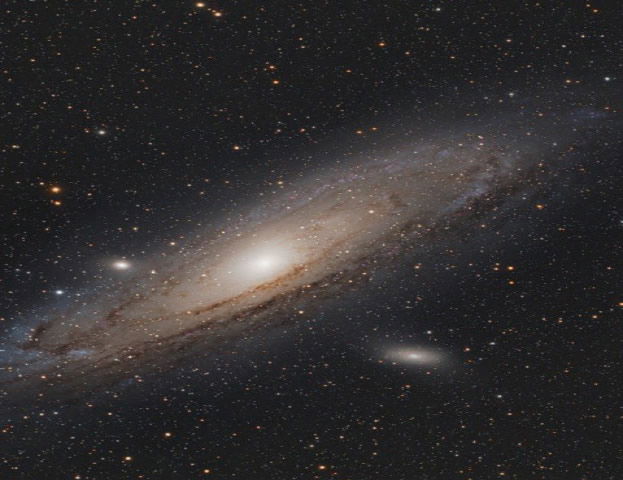
Fig. 2. The Andromeda Galaxy (M31), along with two of its much smaller satellite galaxies. M32 is to the left of the center of M31, while M110 is to the lower right of M31’s center. Photo courtesy of Glen and Katrina Fountain.

The redshifts of galaxies within a cluster have a dispersion in their redshifts centered on an average. Presumably, the average represents the redshift of the cluster, while the dispersion gives us an idea of the typical Doppler motions of galaxies within the cluster. Fig. 2 shows a histogram of redshifts of 42 galaxies in the Coma cluster (Abell 1656). The average redshift is 0.02181, corresponding to a velocity of 6540 km/s, and distance of nearly a hundred Mpc (the established redshift, based upon far more data, is slightly greater, with a correspondingly slightly greater distance). The greatest difference in the redshifts of the galaxies in Fig. 3 is 0.01614, corresponding to a maximum velocity displacement from the average of 2400 km/s. The dispersion is 1000 km/s (Struble and Rood 1999), slightly less than half 2,400 km/s.

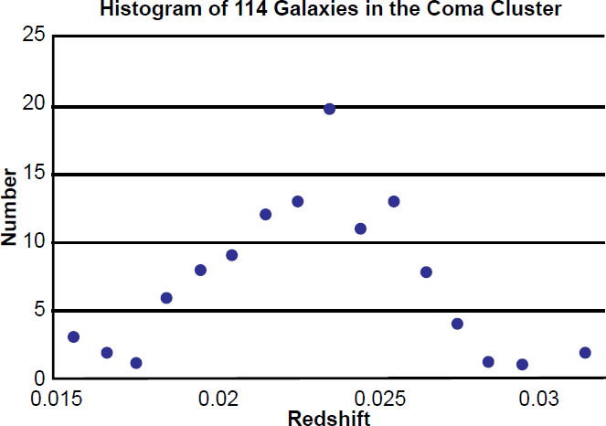
Fig. 3. A histogram of the redshifts of 114 galaxies in the Coma Cluster. The galaxies are all the NGC and IC objects in the Coma Cluster. The redshifts were binned in a range of 0.001 in redshift. Notice the data approximate a Gaussian distribution.

The closest cluster of galaxies is the Virgo Cluster (Fig. 4). The Virgo Cluster contains more than 1000 galaxies and is centered 16.5 Mpc away. Again, assuming H₀ = 70 km/s/Mpc, we would expect the Hubble flow of the Virgo cluster to be 1150 km/s. This is significant, but it probably is comparable to the dispersion velocity of galaxies with the Virgo Cluster. Therefore, the Virgo Cluster cannot be used directly to determine the H₀ (however, it may be used to calibrate more distant clusters). The Virgo Cluster spans about 16° on the sky, corresponding to a diameter of 4.5 Mpc. If the cluster is spherical, the distances of its members range 12–21 Mpc. This places members on the near side of the cluster within range of most standard candles, while those on the far side probably are beyond our ability to measure their distance by most standard candles. All these factors must be accounted for in ascertaining the proper relationship between redshift and distance of these galaxies.

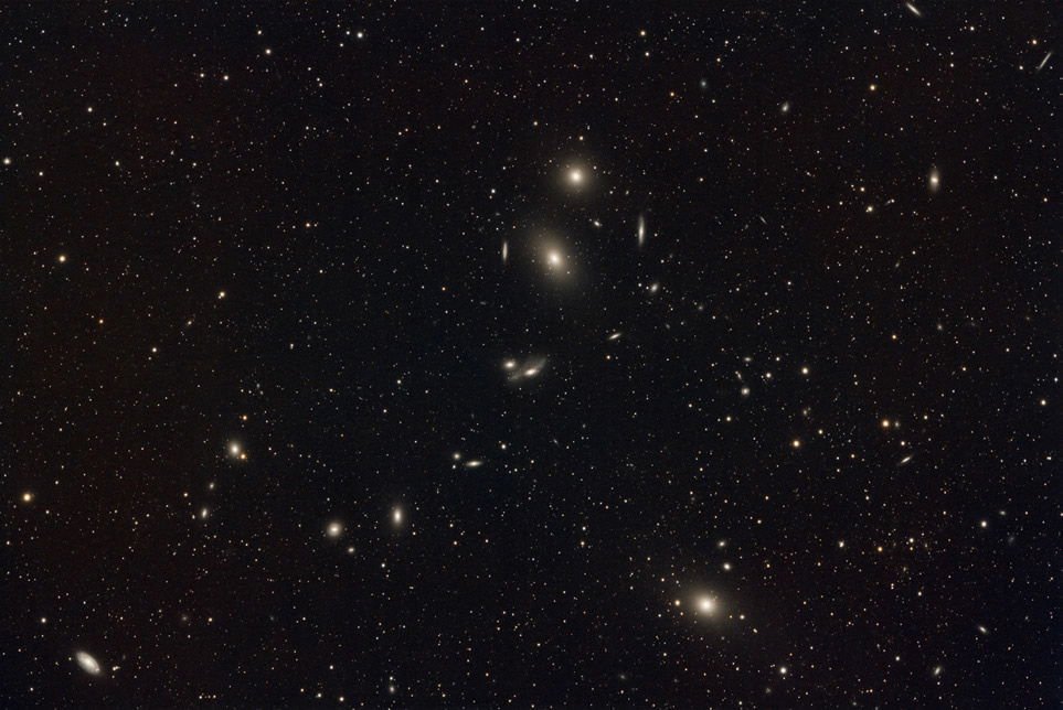
Fig. 4. The central region of the Virgo Cluster. Photo credit: Wikimedia Commons: Kees Scherer.

However, there is a far more significant concern. The Virgo Cluster is so massive that its gravity attracts everything for some considerable distance, including members of the Local Group. Consequently, there is almost certainly a blueshift Doppler component to the redshift we measure for the Virgo cluster. Other nearby galaxies not part of the Virgo Cluster for which we can determine distances by standard candles are attracted toward the Virgo Cluster, almost certainly contaminating their measured redshifts with relatively large Doppler motions compared to their Hubble flow components. How to properly correct for this difficulty has been the source of some of the debate over the value of H₀.

Ideally, one would determine H₀ by measuring redshifts and distances of galaxies so far away that their Doppler component is inconsequential compared to their Hubble flow component. The only standard candle that is bright enough to be used for this is the type Ia supernovae. However, this standard candle has its own unique problem. Type Ia supernovae are relatively rare random events, so the likelihood of seeing one in any given galaxy is quite low. Therefore, this method was of very limited use for some time. However, advances in computer technology have made the type Ia supernovae method of finding extragalactic distances feasible. Robotic telescopes of intermediate size routinely take images of thousands of galaxies every night, and when calibration images are automatically subtracted out, any remaining objects are supernovae. These detections trigger alerts to much larger telescopes that can further investigate whether the supernovae detected are type Ia, measure the maximum brightness of any candidates, and measure the redshifts of the host galaxies. Over the past 25 years, this method has been employed to find redshifts and distances of many galaxies over a broad range of distances and redshifts. Nearly all these measurements are beyond the limit that Doppler components are significant, so the observed redshifts are almost entirely Hubble flow. Therefore, the Hubble relation based upon type Ia supernovae is very robust. This work has been the major method of determining the currently accepted value of H₀ being a little more than 70 km/s/Mpc.

Enter Quasars

The study of extragalactic astronomy underwent a dramatic change in the early 1960s with the discovery of quasars (or QSOs, meaning Quasi-Stellar Objects). Radio surveys of the sky during the 1950s had revealed many radio sources. One of the first orders of business was to identify optical counterparts of these newly discovered objects. Many of the optical counterparts turned out to be nebulae or galaxies. However, a few radio sources did not have any obvious optical counterparts. Eventually, the optical counterparts of some of the radio sources were identified as what appeared to be faint, blue stars. The brightest of these “radio stars,” 3C 273 (the 273rd entry in the Third Cambridge Catalogue of Radio Sources [Edge et al. 1959]), was further investigated in 1963 (Fig. 5). The most prominent features of its spectrum appeared to be Lyman series emission lines redshifted by nearly 16% (z = 0.158). Assuming H₀ = 70 km/s/Mpc, the distance is nearly 700 Mpc (though the value of H₀ at the time, 55 km/Mpc, implied a greater distance). When discovered, 3C 273 was one of the objects with the greatest redshift, and hence the greatest distance (at the time of the discovery of 3C 273, the most distant object known was the radio galaxy 3C 295 with z = 0.461; it would not be until the 1964 discovery of 3C 147, with z = 0.545 that a quasar was the most distant known object). This distance and measured apparent magnitude of 3C 273 indicated that it was about 100 times more luminous than a bright galaxy, such as M31, a galaxy that contains nearly a trillion stars. In other words, 3C 273 outshines more than a few tens of trillions of stars. Even more remarkable, 3C 273 varies in brightness on timescales of decades and even a few days. A variation in brightness requires propagation of some signal related to the physical cause of the variation. The fastest possible signal is light, but physical mechanisms generally are compelled to travel slower than light. Therefore, an object cannot vary in brightness on a timescale that is greater than its size expressed in light travel distance. Therefore, at most, 3C 273 is a few light days in diameter. This makes its maximum size slightly larger than the solar system. Its actual size probably is much less.

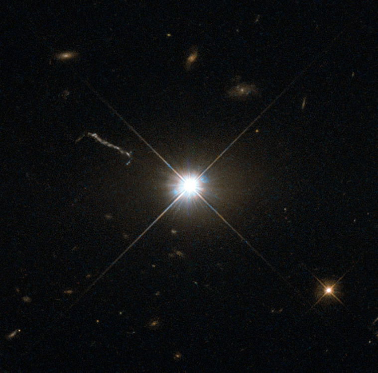
Fig. 5. 3C 273, the first discovered quasar. Photo credit: ESA/Hubble & NASA.

This immediately raised the question of what powers quasars. It was obvious that normal objects, such as stars, would not suffice. The suggestion that quasars are powered by supermassive black holes soon arose. Our understanding of black holes was just emerging in the 1960s (John Wheeler is credited with coining the term “black hole” in 1967). Some people who express doubts about cosmological redshifts for quasars criticize this mechanism, though it often is not clear whether this is motivated more to support the doubts about cosmological redshifts than from genuine concern about the mechanism. At any rate, the details of this mechanism have been fleshed in considerably over the past half-century, a topic I will return to later.

Additional quasars with even greater redshift soon were discovered, and the number of known quasars has increased dramatically over the past half century. The most recent exhaustive catalog of quasars is that of Hewitt and Burbidge (1993), complete until the end of 1992. Their list contains 7315 objects, including about 90 BL Lac objects, which appear related to quasars. Obviously, this list is out of date. More recently, Véron-Cetty and Véron (2010) compiled a list of 133,336 quasars. As one might expect, the discovery of quasars has continued over the past 25 years, and the number of known quasars is far greater today. For instance, the Sloan Digital Sky Survey (SDSS) has resulted in the discovery of many quasars. The SDSS, which has operated since 2000, uses a dedicated 2.5 m optical telescope for an exhaustive imaging and redshift survey of extragalactic objects. The SDSS covers about 35% of the celestial sphere. Myers et al. (2007) culled approximately 300,000 photometrically classed quasars from the fourth data release of the SDSS. Many of these identifications probably were false. While quasars originally were, and are still definitively identified by their large redshifts and point-like appearance, quasars are known to be very blue. Therefore, the easiest way to identify quasars is by their blue color via photometry, which is a much more efficient use of light at the telescope than spectroscopy. However, this method tends to include other non-quasar objects.

More recently, Shen et al. (2011) catalogued 105,783 “bonified” quasars from the seventh data release from the SDSS. If quasars are randomly distributed on the sky (this must be true if quasars are at cosmological distances), and if the SDSS were extended to the entire celestial sphere, it would detect more than 300,000 quasars. If the SDSS is complete (which it is not), there would be, on average, more than seven quasars per square degree of sky. Given the conservative estimates employed here, the actual two-dimensional density of quasars in the sky is probably much higher. This density will be important later.

With the large number of known quasars, astronomers have good understanding of the general characteristics of quasars. I shall discuss some of these later. Furthermore, there have been records for quasars set and then repeatedly broken. One record of interest is the extremes in redshift. Currently, ULAS J1342+0928 is the record holder for greatest redshift with z = 7.54. The quasar 3C 454.3 is the most luminous known object in the universe. Its luminosity is nearly 100 times that of 3C 273. Its redshift is 0.86.

The discovery of quasars rekindled and redirected the debate over the nature of extragalactic redshifts. Much of debate previously had been over the source of redshifts. As previously mentioned, the most straightforward interpretation of the Hubble relation is that the universe is expanding. Universal expansion was anticipated by early cosmologists (for example, De Sitter, Friedman, and LeMaître) who had applied general relativity to the universe prior to or about the same time as Hubble’s discovery of the Hubble relation. In the aftermath of Hubble’s discovery, some astronomers and physicists suggested alternate explanations, such as Zwicky’s tired light hypothesis. This hypothesis proposed that light naturally loses energy as it propagated over large distance, with the amount of energy lost proportional to distance. The mechanism whereby this happened was never identified. Note that this alternative rejected expansion, which was tantamount to rejection of general relativity, upon which the interpretation of the Hubble relation as expansion is based. This alternate explanation for redshifts accepted the reality of the Hubble relation, which is belief that redshifts are cosmological as I have defined it. However, the term cosmological redshift today usually entails not only acceptance that redshifts accurately indicate distance, but also the belief that the universe is expanding.

By the 1960s, this understanding of cosmological redshifts was almost universal. However, by then there had developed two opposing schools of thought on cosmology. One camp embraced the big bang model, the belief that the universe suddenly appeared in the finite past in a very dense, hot state, from which it expanded and cooled to become the universe that we see today. The other camp maintained the eternality of the universe, that the universe had always existed in an expanding state, and it always will. This steady state model, as it came to be called, required the spontaneous creation of matter to maintain a constant average density in the universe as it expanded, so another name for this model was the continuous creation theory. One fundamental difference between these two cosmological models is that a big bang universe has a history, while a steady state universe does not. By this I mean a big bang universe will change with time, while a steady state universe will not. The tremendous distances encountered in extragalactic astronomy suggest look-back time. That is, if an object is a billion light years away, we are now viewing that object as it existed a billion years ago, not as it exists today. Since a steady state universe does not change with time, then there will be no systematic change in what we see at greater distances. But since a big bang universe changes with time, we would expect changes at greater distances with corresponding look-back times.

Quasars presented the steady state model with a problem of crisis proportions. There are no low redshift quasars, which, if redshifts are cosmological, suggests that quasars do not exist locally. Furthermore, within four years of their discovery, it was shown that the density of quasars increases with increasing distance. This suggests that quasars were abundant in the past, but are relatively rare today, implying that the universe has a history. Ergo, the existence of quasars, if their redshifts are cosmological, disproves the steady state theory. Therefore, it is no wonder that the harshest critics of redshifts of quasars being cosmological (for example, Arp, Burbidge, and Hoyle) also were proponents of the steady state model. In 1965, halfway between the discovery of quasars and recognition of their implications about the history of the universe, was the discovery of the cosmic microwave background (CMB). While the CMB is often credited with the demise of the steady state model, it likely was the one-two punch of the CMB and the history implications of quasars that did that model in. The major opponents of redshifts of quasars being cosmological have died, and with them much enthusiasm for this opposition died too.

Recent creationists came to this discussion a little late, but many creationists long have criticized the Hubble relation (Bouw 1982; DeYoung 1983; Ettari 1988). The motivation appears to have been opposition to the big bang cosmology. The belief appears to be that if the universe is not expanding, the big bang model cannot be true. That is correct, but acceptance of expansion of the universe does not inevitably lead to the big bang model. For instance, the steady state model was based upon universal expansion too. What if the universe truly is expanding? If we reject that out of hand, then we have no hope of establishing a proper biblical cosmology. Other responses by recent creationists apparently accept the reality of the Hubble relation, but attempt to explain it by means other than universal expansion (Bishard 2006; Hartnett 2002, 2005d, 2011a, 2011b; Oard 1987; Repp 2003). Much of this has focused on alternate explanations for high redshifts of quasars (Worraker 2006). For instance, Hartnett (2005a, 2005b) has suggested that the Hubble relation is a result of God stretching space.

It is not clear what motivates this thinking. Some of these writers apparently do not understand that rejection of cosmic expansion is tantamount to rejection of general relativity. Recent Creationists often use the possibility that redshifts may be quantized as evidence that we are at the center of the universe (Humphreys 2002). Incidentally, in this paper Humphreys opined that after spending many years opposing universal expansion as the cause of the redshifts, he eventually came to accept some form of expansion as the cause. However, many other recent creationists failed to come to this conclusion. Consequently, some recent creationists express doubts about reality of the Hubble relation and cosmological redshifts while simultaneously embracing the galactocentric implications of quantized redshifts without realizing the inherent contradiction of these two positions. Much of this discussion of redshifts in the creation literature centers on the nature of quasars. For instance, Hartnett (2003, 2004a, 2004b, 2005c) argues that quasars are ejected from cores of relatively nearby galaxies and hence are much closer than generally thought (this is very similar to what Arp had argued, albeit invoking a different mechanism—Hartnett suggests that we may be witnessing Day Four creation of these objects) Much of this seems muddled, which is why this review of redshifts and quasars in the creation science literature is so needed.

The Work of Halton Arp

Key to this discussion is the work of the late astronomer Halton Arp. Early in his career, Arp distinguished himself as a keen observer, a veritable giant in the field of observational astronomy. Arp’s most notable publication was his Atlas of Peculiar Galaxies (Arp 1966). However, Arp soon focused his attention on questioning cosmological redshifts. He actively pursued this work for two decades, but by the 1980s, most astronomers had concluded that Arp’s work on this was pointless, and it was taking up valuable large telescope time that could otherwise be used for more productive studies. This led to the directors of the Palomar Observatory and National Optical Astronomy Observatory collectively informing Arp that he no longer would be granted telescope time at either institution to pursue this work. Arp was free to pursue other types of research, but not the type of work he had dedicated his life to. Since there were no other appropriate observatories available to him, Arp considered this move outrageous. He retired and took a position at the Max Planck Institute for Astrophysics in Germany, where he remained the rest of his life. Understandably, this experience embittered Arp, and he shared his thoughts about this, as well as his life’s work in two books aimed at popular-level audiences (Arp 1987, 1998). These two books are well-known by recent creationists who doubt that redshifts are cosmological. Less well known are two, more technical, books by Arp on the subject, one published early (Field, Arp, and Bahcall 1973), and one that was Arp’s last book (Arp 2003).

A major part of Arp’s argument against cosmological redshifts was the identification of pairs of objects that form optical images that appear to be connected by matter yet have discordant redshifts. If a pair of objects truly are connected, then they must be at the same distance. But if redshifts are cosmological, then the discordant redshifts of the pair indicate radically different distances. Hence, if one can establish even one unequivocal interacting pair of extragalactic objects with discordant redshifts, then the cosmological interpretation of redshifts is in doubt. The best-known example of this is the spiral galaxy NGC 4319 and the Seyfert-like object Markarian 205 (this pair is so important, a highly processed image of the two graces the dust jacket of Arp’s 1987 book). Arp (1971) published a four-hour photograph using the 200-inch Hale Telescope (then the largest telescope in the world). The photograph shows what appears to be a luminous bridge connecting the two objects. Arp reported that the redshift of NGC 4319 was 1700 ± 100 km/s, while Weedman (1970) previously reported a redshift z = 0.070 (corresponding to a velocity of 21,000 km/s) for Markarian 205.

If the redshifts involved are cosmological, then Markarian 205 is more than ten times more distant than NGC 4319. If the luminous bridge were real, then this would be a damaging counterexample to cosmological redshifts, but is the bridge real? Much discussion in the astronomy literature ensued, with most critics contending that the bridge was due to overlap of the images of the two objects involved, with inevitable bleeding in the emulsion. Both sides seemed confident of their conclusions. Arp’s original claims were based upon images taken on photographic plates. Photographic plates long ago were replaced by far more sensitive CCD chips. Furthermore, larger telescopes, advancements in telescope design, such as adaptive optics, and the Hubble Space Telescope (HST) from its location above the earth’s atmosphere give us far better images to assess these claims. For instance, the in HST photo of NGC and Markarian 205 (Fig. 6), there is no luminous bridge present. Furthermore, Bahcall et al. (1992) obtained a near-ultraviolet spectrum of Markarian 205 indicating absorption due to material in NGC 4319. Thus, Markarian 205 is a background object to NGC 4319, in line with the redshifts of the two objects being cosmological. Since the best example of Arp’s physically connected objects having discordant redshifts are indeed not connected, it does not bode well for his other, more tenuous, examples.

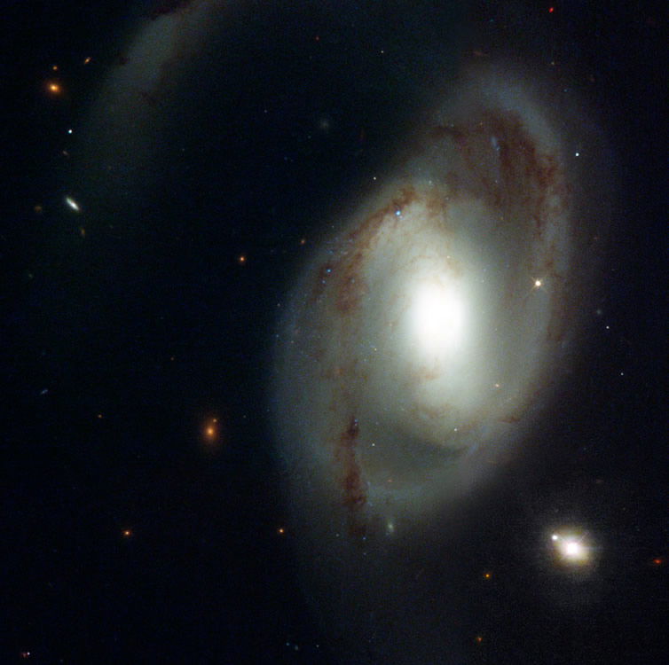
Fig. 6. NGC 4319 and Markarian 205 (lower right). Notice that there is no clear evidence of a luminous bridge between the two. Photo credit: NASA/ESA and The Hubble Heritage Team (STScI/AURA).

If quasars are not extremely luminous objects at great distances, what does Arp suggest they are? Arp proposed that relatively nearby galaxies eject quasars from their cores. In Arp’s assessment, quasars may be the sites of newly created matter required in the steady state cosmology. Presumably, the large redshifts of quasars are Doppler motions of this ejection. Why do quasars all have redshifts, suggesting that all of them are moving away from us? Would we not expect to see about as many quasars directed toward us, with large blueshifts? Arp proposed that ejected matter directed toward us is not visible. Perhaps the redshifts are a sort of exhaust, while in approaching quasars, no radiation is visible.

Arp found instances of quasars clumped around galaxies that he suggested were examples of this ejection mechanism. Simultaneously, Arp has argued these examples of quasar clumping around galaxies are evidence that quasar redshifts are not cosmological. This generally is based upon statistical grounds that quasars are unlikely to be seen clumped around a galaxy, if the galaxy and quasars merely are along the same line of sight but at much different distances. On the other hand, such clumping would be expected if quasars are associated with the galaxy despite their discordant redshifts.

A good example to discuss is one previously described in the creation literature (Hartnett 2005c). Galianni et al. (2005) announced the discovery of a quasar with z = 2.114 located only 8˝ from the center of NGC 7319, a member of Stephan’s Quintet having z = 0.022 (Fig. 7). If these redshifts are cosmological, then then the quasar is a much more distant object that merely is in the same direction as the galaxy. Since the quasar appears embedded in the luminous portion of the galaxy where a spiral arm leaves the nucleus, one might expect that if the quasar is far beyond the galaxy, there ought to be absorption in the quasar’s spectrum from gas within the galaxy. Indeed, Galianni et al. tested for this, and they found evidence of absorption, but they reasoned that this could be explained if the quasar lies within the disk of the galaxy or just beyond the disk. Notice carefully what is going on here. If there were no absorption from gas in the galaxy in the spectrum of the quasar, that would be evidence for Arp’s contention. But if there is absorption, then that can be explained by Arp’s contention too. Therefore, Arp’s contention can account for evidence either way. That is, Arp’s hypothesis makes no testable prediction in this matter. However, the conventional understanding, that the quasar is a background object, makes a very specific prediction that was tested, and it passed that test. Arp and his supporters have set up a test that is meaningless about their theory, because it can pass the test either way.

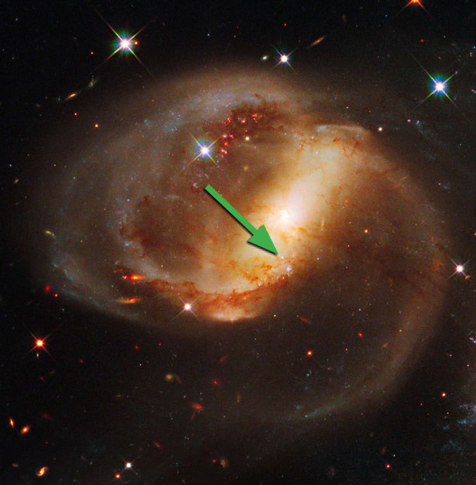
Fig. 7. HST photo of NGC 7319. The arrow indicates the location of the quasar. Photo credit: NASA, ESA, and the Hubble SM4 ERO Team.

Since the spectral absorption data was inconclusive according to Galianni, et al., they moved on to a statistical alignment argument. They gave an equation for the probability, p, that a quasar would lie within an angular distance, θ, of a point, given the two-dimensional density of quasars per square degree, Γ:

They accepted as well established that Γ ≈ 5–10 per square degree down to magnitude 20 and leveling off at ≈ 50 per square degree for magnitude 21. These values are consistent with what I reasoned above. Using the lower value of Γ, Galianni, et al. concluded that the probability of finding the quasar within 10˝ of the center of the galaxy was 10^-4, while using the higher value of Γ yields a probability of 10^-3. Since this is a low probability, the authors concluded that this likely is not a chance alignment.

This sort of calculation and reasoning has been very important in Arp’s argument of clumping of quasars around galaxies for years. But how sound is this conclusion? In using probability, how one frames the question is very important. For instance, the probability of flipping a fair coin so that it comes up heads five times in a row is (1/2)⁵ = 1/32. However, what is the probability that the fifth flip will come up heads, given that the previous four flips all were heads? To many people not knowledgeable about probability, the answer is a surprising ½. While the two questions posed may appear very similar, they are very different questions, so the resulting probabilities are very different. In the case of the clumping of quasars around galaxies of lower redshifts, Arp and his colleagues first found the distribution of the quasars and galaxies in the sky and then asked what the probability of this happening by chance was. Since the distribution happened, its probability was one. The probabilities they cite make sense only if one asks the probability of a given distribution prior to finding the distribution.

Look at it another way. Given the way genetic material is shuffled during reproduction, the total possible number of unique children that any couple can have is staggering. Yet, human couples can have only a very small number of children. Therefore, one could conclude that the probability of any one of us existing is vanishingly small, yet here we are. Of course, the resolution to this paradox is that each one of us happened, so the probability that each one of us happened is one. This sort of statistical argument works only if one specifies the outcome prior to investigating the outcome. Asking the probability after the outcome is determined is meaningless.

Applying this reasoning to the distribution of quasars and galaxies in the sky, each distribution one finds, those with close clumping of quasars around galaxies, and those that are not clumped, are equally improbable. Arp and his colleagues have unintentionally biased their searches toward finding clumping of quasars with galaxies. This amounts to cherry-picking data. If both quasars and galaxies are somewhat randomly distributed in space, then it would be amazing if there were no clumping found. Indeed, if after extensive searching, no clumping of quasars and galaxies were found, that would indicate that something peculiar was going on.

Lyman-Alpha Forests

One of the major arguments for quasar redshift being cosmological is the Lyman-alpha forest in the spectra of many quasars (Fig. 8). This phenomenon was discovered by Lynds (1971) in the spectrum of 4C 05.34, at the time the greatest redshift object known (z = 2.877). Lyman-alpha absorption arises from the transition of electrons between the ground state and the first excited state in hydrogen atoms. Its rest wavelength is 121.6 nm, which is deep in the ultraviolet. To see Lyman-alpha absorption requires two things:

1. a more distant bright ultraviolet continuum source
2. nearer clouds of cool hydrogen atoms along the line of sight to the continuum source.

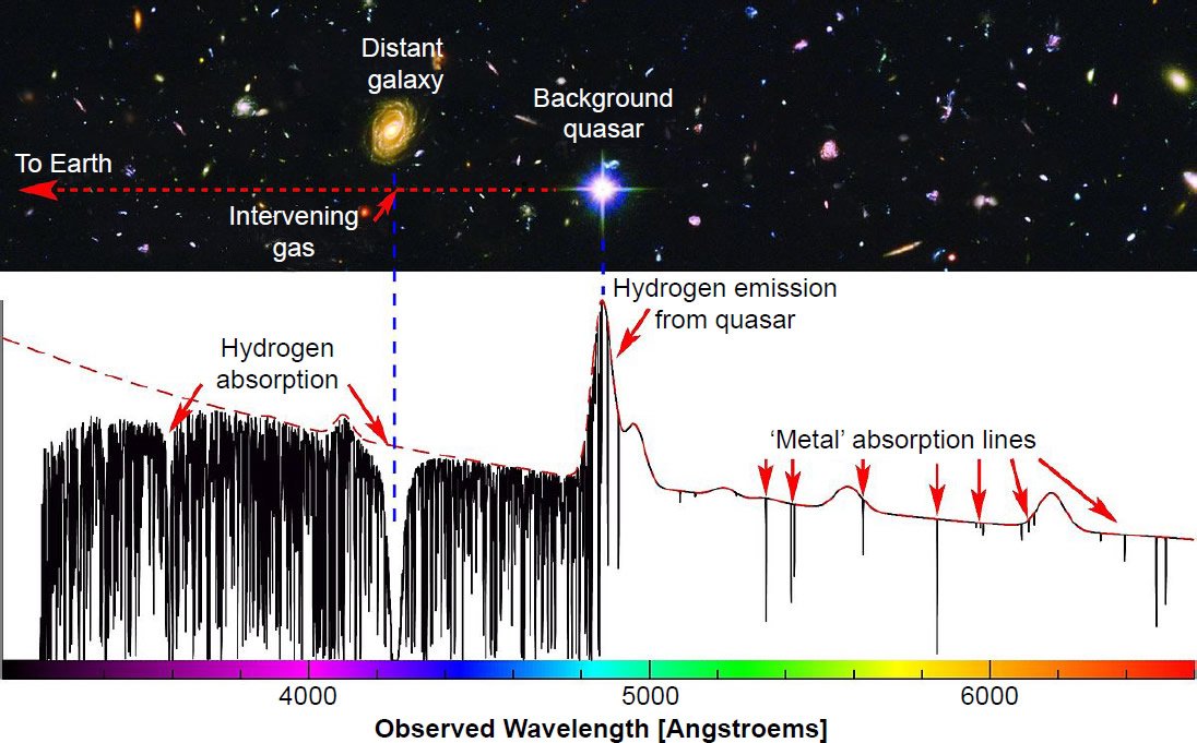
Fig. 8. A schematic diagram of the Lyman-alpha forest. A typical quasar spectrum is illustrated in the lower portion. The spectrum is dominated by a hydrogen emission line (in the middle, at approximately 4800 Angstroms wavelength. Notice the metal absorption lines to the right (at longer wavelengths). There are hydrogen absorption lines left (at shorter wavelengths) of the hydrogen emission line. The top portion of the diagram illustrates how intervening clouds at lower redshift produce this absorption. Image credit: Joel Liske, European Southern Observatory.

Regardless of their distance, quasars have bright ultraviolet continua. The cool hydrogen clouds cannot be near the quasars, because if they were, the ultraviolet continuum of the quasars rapidly would ionize and heat the hydrogen, leaving no appreciable number of hydrogen atoms in the ground state to produce Lyman-alpha absorption. Quasars typically have multiple Lyman-alpha absorption of various strengths and at various redshifts, but always with redshifts less than the quasars themselves. These multiple absorptions are the reason for the term Lyman-alpha forest.

If quasar redshifts are cosmological, then the existence of Lyman-alpha forests in their spectra has a very simple explanation. Hydrogen is the most abundant atom in the universe, and clouds of cool hydrogen have been known to exist within galaxies and in the intergalactic medium for some time. Therefore, as the light of a very distant quasar travels toward earth, we would expect it to pass through many of these cool hydrogen clouds. Each cloud would absorb energy at λ = 121.6 nm in its reference frame as hydrogen within the cloud transitions from the ground state to the first excited state. However, since each cloud is subject to the Hubble relation (whether due to expansion or to some yet unknown process), the Lyman-alpha absorption would be redshifted by the redshift of each cloud. Since all the clouds are closer than the quasar, the Lyman-alpha absorption lines have less redshift than the Lyman-alpha emission of the quasar. This is what we consistently see—Lyman-alpha absorption always is redshifted less than the Lyman-alpha emission of the quasar. This is a key point, because the absorption is possible only if the absorbing regions are closer than the source of the continuum (Kirchoff’s third law of spectroscopy). This is a powerful argument that the Hubble relations holds for all sorts of extragalactic objects over a wide range of redshifts.

Quasar Properties

As previously mentioned, the most distinctive quality of quasars is their high redshifts. Quasars emit across most of the spectrum from x-rays to radio (though some are radio quite). The peak emission typically is in the near ultraviolet and optical. Some quasars are sources of gamma rays. All the early discovered quasars were quite bright in the radio part of the spectrum, which is what flagged their discovery. However, after more than a decade, astronomers began to find radio-quiet quasars. The most often used method of detection of quasars now is by their distinctive very blue color in optical images. In optical images, quasars appear as stars, indicating their small size (distant galaxies appear as much less blue smudges). Galactic blue stars are confined to the galactic plane, while quasars are not found at low galactic latitudes. Hence, very blue stars at any appreciable galactic latitude almost always are quasars. The definitive test is to measure redshift of quasar candidates. The optical spectrum is characterized by hydrogen emission lines, something again not found in stars. These emission lines typically are from the Lyman series normally found in the ultraviolet but redshifted to the visible. Measurement of the wavelength of the Lyman emission lines compared to the rest wavelength provides z. In addition to hydrogen lines, emission lines of other atoms, most notably helium, carbon, oxygen, magnesium, and iron, are also present. The lines are Doppler broadened, indicating high average speed in the emitting region. This implies large mass. The emission lines range from neutral atoms to highly ionized atoms. This wide range indicates the gas is not merely hot, nor is it illuminated by radiation from stars. The spectra of quasars are decidedly non-thermal, again a departure from stars. Overall, the spectra of quasars best conform to a synchrotron spectrum, indicating powerful magnetic fields and fast-moving charged particles. This, too, is an important clue in deciphering what is going on in quasars. Some quasars have jets. These jets may be singular, or there may be two jets. When in pairs, the jets appear to go in opposite directions.

Many of the properties just described are shared with active galaxies, though the activity in quasars is far higher. For instance, Seyfert galaxies appear as normal spiral galaxies in most photographs. However, the point-like blue cores of Seyfert galaxies are very intense. Their total luminosity at all wavelengths can exceed the output of the rest of the galaxy. Like quasars, Seyfert galaxy cores have emission lines of various elements showing many different levels of ionization. They have strong Doppler broadening, again demonstrating high velocity from the emitting region. Seyfert galaxies sometimes have jets. These similarities with quasars suggest a common mechanism behind them. Seyfert galaxies and their nuclei have the same redshifts, so no one disputes that the two are related. Seyfert galaxies generally have much lower redshifts than quasars. Because of their point-like energetic nature surrounded by a galaxy, both Seyfert galaxies and quasars are grouped together into a class of objects that have an active galactic nucleus, usually abbreviated as AGN.

While many quasars and Seyfert galaxies have relatively little or no observable radio emission, some of them are quite energetic in the radio part of the spectrum. This intersects with another class of galaxies, radio galaxies. Galaxies normally have some radio emission, probably from the collective contribution of sources within them that produce radio emission. In a normal galaxy, this radio emission is a small fraction of the total luminosity of a galaxy. However, radio galaxies have inordinately high radio emission, typically dwarfing their optical emission in power. Most radio galaxies are ellipticals rather than spirals. They frequently have a jet or two oppositely directed jets emanating from their cores, with material in the jets moving at relativistic speeds. These jets can extend considerable distance from the galactic cores. At the termination of a jet there often is a large lobe of radio emission. These lobes often dwarf the galaxy in size.

The best example of a radio galaxy is M87, a giant elliptical galaxy at the center of the Virgo Cluster. Given its large size, M87 probably is the most massive galaxy within a distance of tens of Mpc. It has a single jet that appears blue in color photographs, which contrasts with the much redder stars in the galaxy. There probably is an oppositely directed jet that we cannot see. Knots in the jet are superluminal, meaning that they are moving faster than the speed of light. However, this is an illusion caused by a relativistic effect due to the jet having a large component of motion in our line of sight. The jet extends several times the diameter of the Milky Way galaxy. Both the polarization and synchrotron spectrum of the jet indicate that the jet is generated by electrons moving with relativistic speed in a powerful magnetic field. M87 is bright across the entire spectrum, being a very strong source of x-rays and gamma rays. Its core is very active, qualifying M87 as an AGN.

Another type of AGNs are BL Lacertae (usually abbreviated as BL Lac) objects. BL Lac is a variable star designation. This is because when BL Lac, the prototype of this class, was discovered in 1929, its point-like nature and rapid brightness variations led astronomers to think it was an irregular variable star. Its true nature as an AGN was not learned until four decades later. The cores of BL Lac objects are characterized by large amplitude rapid brightness variations, larger amplitudes and shorter periods than other AGNs. They typically lack the broad emission lines of quasars. In fact, the spectra of BL Lac objects usually are featureless non-thermal emission. The lack of spectral lines often makes determination of redshift, and hence distance, difficult. The host galaxies of BL Lac objects appear to be giant ellipticals.

Making Sense of the Zoo

A half century ago, the field of AGN studies in astronomy was in its infancy. Since then, the field has matured tremendously, though few recent creationists seem to be aware of this. My brief discussion of AGNs here should not be taken as anywhere near exhaustive. For many years, AGNs appeared to be grouped into distinct bins of odd objects, amounting to a sort of zoo. However, as more was learned about AGNs, some common themes began to emerge, and instead of seeing different AGNs as distinct objects requiring different explanations, a single unifying theory has emerged. I shall now briefly describe the current understanding of AGNs.

First, I should note that by the 1970s, astronomers began to suspect that quasars were in the cores of very distant galaxies. It was difficult to demonstrate this at first, because of the limits of observations at the time. However, eventually images of some quasars began to show that they were surrounded by luminous fuzz that appeared to be the outer regions of galaxies. Over the years, this contention has strengthened considerably with huge amounts of new data. Whereas quasars and galaxies originally were thought of as distinct objects, quasars now are grouped with other AGNs. Interpreting their high redshifts as cosmological indicates that quasars are very far away. Understanding great distance as great look-back time, quasars must be galaxies in their infancy. Other AGNs generally have much lower redshift, and hence must be much less distant than typical quasars. Therefore, other AGNs probably are more mature galaxies.

Despite some differences in various types of AGNs, they all share one common property: extremely high luminosity coming from very small volumes. What mechanism can account for this excessively high power density? Astrophysicists have given this problem considerable thought over the past half century, and only one possible mechanism has been identified: supermassive black holes. Black holes are regions of space containing so much mass in so little volume that the escape velocity exceeds the speed of light. The Schwarzschild radius is the distance from the center where the escape velocity is equal to the speed of light. The surface having radius equal to the Schwarzschild radius is the event horizon. The event horizon effectively defines the boundary of a black hole—material and light within the event horizon cannot escape, while matter and energy outside the event horizon may escape. Like an expanding universe, cosmological redshifts, and quasars, many recent creationists express doubts about black holes. However, there are good observational reasons for the existence of black holes (Faulkner 2007).

Presumably, a black hole is surrounded by matter, some of which probably orbits the black hole. Orbiting material may have different orbital planes, making mutual collisions of the orbiting matter inevitable. Collisions rob the matter of orbital energy, forcing the matter to lower orbits. However, orbital speed is inversely proportional to the square root of orbital distance (v = [2GM/r]^1/2). Therefore, counterintuitively, infalling matter increases its orbital speed. Furthermore, as orbital distance decreases, so does the volume the orbiting bodies can occupy (volume is proportional to the third power of the radius, so halving the orbital distance decreases the volume to 1/8 its original size). Both increasing speed and smaller volume available increases the likelihood of collisions, so the infalling process proceeds at an ever-increasing rate. Furthermore, the collisions tend to cancel opposing directions of motion, so the infalling matter tends to collapse into a disk representing the plane of the average of most of the original motion.

What happens to the lost orbital energy? Most of it is converted into random microscopic motion. Since we interpret random microscopic motion as heat, the temperature in the disk increases. We say the orbital motion is thermalized. The gravitational potential well of a black hole is so deep and steep, the temperature of the disk can be very high (millions of K). Even if most of the infalling material originally was not gaseous, the exceedingly high temperatures achieved eventually will convert all of it to gas. The innermost part of the disk is the hottest, hot enough to produce copious x-rays. Large amounts of x-rays are difficult to produce, so when astronomers detect them, it gets their attention. This is the way that stellar-sized black holes are detected. If a black hole exists in close binary star with its companion being a normal star, tides raised on the normal star by the black hole can lift matter from the normal star and transfer it to the black hole. Conservation of angular momentum prevents the matter from transferring directly to the black hole. Instead, the matter forms a disk around the black hole, from which it slowly spirals down onto the black hole. Astronomers have detected many x-ray binaries. Applying Newtonian gravity to the orbital motion allows astronomers to measure the mass of the unseen member of such binary stars.5 When the mass of the object in question is within the range expected of a black hole, presumably it is a black hole (the other possibility is a neutron star, but its mass is less than that of a black hole). There are many known stellar black holes having mass in the range of 4–20 times the mass of the sun, but new gravitational wave detections of black holes have extended this to much higher masses.

Matter that falls into a black hole, whether during formation or later, often possesses magnetic fields. These fields are conserved, but when magnetic fields are compressed into smaller volume, the intensity of the magnetic fields increase. Since black holes are extremely small objects, we expect them to have very strong magnetic fields. Matter orbiting outside the black hole is so hot that it is highly ionized, meaning that there are many charged particles present moving at very high speeds. Therefore, there will be large relative motion between the magnetic field and the charged particles. Relative velocity between charged particles and a magnetic field results in acceleration of the charged particles. This can produce a jet of matter emanating perpendicular to the disk, typically in opposing directions Where does the kinetic energy of this motion come from? It comes at the expense of other matter that is driven to lower orbits, ever closer to the black hole event horizon. Therefore, this is a very efficient engine that can selectively remove some matter from the vicinity of the black hole with very high velocity. This phenomenon of jets has been detected in stellar-sized black holes within our galaxy. Computation shows that the mass range of black holes required to power AGNs of all types are in the range of millions of times the mass of the sun, hence the name, supermassive black holes, to distinguish them from stellar-sized black holes.

The masses of black holes at the hearts of AGNs almost certainly vary, and the mass of the black hole involved in any AGN would affect its output, but this is just one parameter. Another parameter is the magnetic field strength. Another obvious parameter is the rate of infalling matter. A supermassive black hole starved of infalling matter will not be very luminous, while one with a huge influx of matter would be much brighter. The properties of the disk are important as well. The disk can be very thin, or it can be very thick. Only the innermost regions have high temperatures—the outermost regions can be much cooler. A thick disk tends to focus any jets present, while a thin disk allows for the jets to be much broader. Finally, the orientation of the plane of the disk (and the jets, since they are perpendicular to the disk) is vitally important. If we view an AGN near the plane of its disk, the view of the inner portion of the disk will be obscured. However, if our view of an AGN is perpendicular to the plane of its disk, we most easily can see the inner portion of the disk. Furthermore, this orientation means that one jet is pointing directly at us. For orientations near perpendicular to the disk, the jet in the other direction is almost certainly obscured by the disk. This is part of the explanation of why we sometimes see only one jet in AGNs. For various orientations, what we see will be different, even if all the other parameters were the same.

Astronomers now invoke this single theory, but with different parameters in individual cases, to explain various AGNs. For instance, BL Lac objects are thought to be examples of our line of sight being perpendicular to the plane of the disk so that we are peering down one jet. The difficult-to-classify M87 appears to be oriented so that we view its central engine at a high angle to its disk, but not perpendicular. Consequently, M87’s oppositely directed jet is obscured mostly by the galaxy. What about quasars? Being the brightest, most distant, and hence having the greatest look-back time, quasars are interpreted as being hosted in very young galaxies. Apparently, high core luminosity is a characteristic of galaxies in their youths. Perhaps with age, AGNs become starved of infalling matter and fade into obscurity.

What about the Milky Way and other nearby galaxies that appear normal, that is, their cores are not blazingly bright? Despite relative quiescence, things are not quite so normal in a supposedly normal galaxy. For a long time, astronomers suspected that a supermassive black hole was lurking at the center of the Milky Way, but this is now confirmed. Probing this portion of our own galaxy is difficult, because of obscuring dust in the plane of the galaxy. However, radio waves penetrate through the dust relatively easily, and modern radio astronomy instruments and techniques have revealed much that is going on there. Radio astronomers have measured orbital motion of objects very close to the center of the galaxy. The mass required explain to the orbits is on the order of 3 million times the mass of the sun (Worraker 2005). The maximum dimension of this mass is only 17 light hours, requiring the existence of a 3 million solar mass black hole at the galaxy’s center. The HST and other breakthroughs in optical astronomy have permitted similar studies in other nearby galaxies, producing observations strongly indicating the existence of supermassive black holes at the centers of nearly every large nearby galaxy. The most extreme case is the galaxy M104, with its core black hole containing a whopping billion times the mass of the sun (Kormendy et al. 1996). Within the evolutionary scenario, it would appear that the black holes in the centers of “normal” galaxies are no longer being fed, so there are no large emissions radiating from them.

Discussion

Given the strong case for redshifts, including those of quasars, being cosmological, why do so many recent creationists resist it? There are at least four possible reasons. One reason is that most recent creationists appear to be ignorant of the tremendous amount of data that has accumulated over the past half century in support of redshifts of quasars being cosmological. Hence, this resistance is decades out of date. Since few recent creationists are astronomers, this ignorance is understandable. I chose to write this review to help overcome this shortcoming. Such a review has been lacking in the creation literature for decades.

A second reason is that within any movement, including that of biblical creation, there is a certain amount of herd mentality. The modern recent creation movement began in the 1960s, just as quasars were discovered. Over the next decade, astronomers began to understand quasars better. With this new understanding, some influential recent creationists expressed doubts about the Hubble relation, expansion of the universe, and whether quasars truly were very distant objects. I have had difficulty finding any sources in the creation science literature that were positive about these things, but there were many which were not. Given this one-sided view, it is not surprising that there is so much skepticism about cosmological redshifts among creationists. Again, this underscores the need for a review such as this.

Why did early modern recent creationists oppose cosmological redshifts? That brings up a third reason. There is a tendency of recent creationists to treat with skepticism many pronouncements of mainstream scientists. Given the widespread belief in evolution of all types in mainstream science, some level of caution is always warranted, for evolutionary assumptions could be hidden away within many things that may seem otherwise innocuous. However, one must be careful that healthy skepticism does not give way to an attitude of, in the words of Yosemite Sam, “If’n he’s fer it, then I’m agin it!” Such a knee-jerk reaction easily can result in rejecting concepts that are correct and even useful in developing a creation model. Instead, claims and discoveries must be evaluated carefully and responded to effectively.

The fourth reason why so many recent creationists are opposed to cosmological redshifts is that denial of an expanding universe is a short-cut to undermining the big bang model. The big bang model was developed in response to recognition that the universe is expanding. Therefore, if the universe is not expanding, then the big bang model cannot be true. However, belief in an expanding universe does not inevitably lead to the big bang model. Indeed, the steady state model also relied upon an expanding universe, and there was much more support for the steady state than for the big bang model in the first three decades after Hubble’s 1929 discovery. There are many other cosmologies one could spin based upon an expanding universe, including ones based upon biblical creation. One such example was Humphreys’ (1994) white hole cosmology. What if the universe truly is expanding? Rejection of that would doom any attempt to develop a proper biblical cosmology.

There are three questions or issues that must be addressed, the same three questions raised in the Introduction. The first question is whether the universe is expanding. The most straightforward interpretation of the Hubble relation is that the universe is expanding. However, this is an interpretation, not direct proof. Early on, some astronomers and physicists pursued alternate explanations for the Hubble relation, but in nearly a century, nothing has become of this. If the universe is not expanding, then it remains a mystery why the Hubble relation appears to describe the universe very well. Before Hubble’s discovery, cosmologists who had applied general relativity to the universe had anticipated expansion. General relativity predicted that in the general case, the universe was either expanding or contracting. It was a matter of observation to determine which possibility was the correct description of the universe. Therefore, denial of the expansion of the universe interpretation of the Hubble relation amounts to a denial of general relativity. This is profound, because some recent creationists who doubt that the universe is expanding appear to have no problem with general relativity.

Furthermore, contrary to common misconception among recent creationists, Arp and other astronomers who questioned whether quasars had cosmological redshifts never doubted that the universe was expanding. Indeed, Arp and his colleagues clung to the steady state model long after nearly everyone else had abandoned it. The steady state model is not possible if the universe is not expanding, so it would have made no sense for Arp and his colleagues to have doubted universal expansion. Consequently, Arp’s work is greatly misunderstood in the recent creation community.

The second question is whether the Hubble relation is real, at least as applied to galaxies. That is, is there a linear relationship between galaxy redshift and distance? The resounding answer is yes. Since Hubble’s pioneering work nearly a century ago, astronomers have greatly improved and extended the Hubble relation. The Hubble relation is very robust. Therefore, even Arp, who has been a leading figure in the discussion here, accepted the reality of the Hubble relation, because he accepted the idea of an expanding universe (many recent creationists who praise Arp’s work seem to be unaware of this). Hence, denial of the Hubble relation is not an option for recent creationists.

This leads to the third question: are quasar redshifts cosmological? While most astronomers believe that quasar redshifts are cosmological, Arp resoundingly argued otherwise. Arp thought that most redshifts of extragalactic objects were cosmological, but he thought it was a slavish mentality to assume that all extragalactic redshifts were cosmological. Arp produced numerous examples of what he thought were physically connected galaxies and quasars with discordant redshifts. He also found what he thought were physically connected pairs of galaxies with discordant redshifts. However, there are far more examples of physically connected galaxies with the same redshift. For instance, many entries in Arp’s Atlas of Peculiar Galaxies appear to be interacting galaxies, yet they have similar redshifts. Therefore, it appears that Arp cherry-picked many of his examples of supposedly interacting objects with discordant redshifts. Again, Arp believed that most redshifts were cosmological, but that there were exceptions. Who was to decide what the exceptions were? Well, of course, Arp decided.

As previously mentioned, Arp appears to have been motivated by the need to salvage the steady state model. If quasar redshifts are cosmological, then quasars are very distant objects, and there are no local quasars. If extragalactic distances reflect light travel time distances, then vast distances equate with vast look-back times. Therefore, quasars must have existed in the early universe, but they do not exist today. This leaves one with the conclusion that the universe has changed, or evolved, over time. However, in the steady state model, the universe is eternal, and so the universe does not evolve. Therefore, within a naturalistic worldview, recognition that quasar redshifts are cosmological leads one to abandon the steady state model. This fact, along with the 1965 discovery of the CMB, was responsible for the abandonment of the steady state model, except for a minority, including Arp. For those who clung to the steady state model, it became necessary to deny that quasar redshifts are cosmological. Recent creationists who celebrate Arp’s work generally fail to recognize Arp’s philosophical bias. This is in addition to the failure to understand that Arp did not doubt that the universe is expanding.

A half century ago, quasars and galaxies appeared to be distinct things. However, astronomers soon began to suspect that quasars might be caused by unusually strong activity in the cores of galaxies, usually interpreted as galaxies in their infancy. This suspicion eventually was confirmed, as deeper photographs revealed that many quasars are surrounded by light fuzz consistent with that interpretation. A unified theory of supermassive black holes began to emerge to explain not only quasars, but also “unusual” galaxies, such as those with AGNs. This model has been very successful. Furthermore, the discovery of supermassive black holes in the cores of otherwise unremarkable galaxies has undermined the concept of “normal” galaxies, as that term was understood a half century ago. It now appears that the distinction between quasars and so-called normal galaxies is artificial, representing the extremes of galaxies possessing the most energetic and least energetic cores. This important development went by almost without comment from Arp, who continued to concentrate on quasars as if they were objects distinct from galaxies. This has passed the notice of most recent creationists as well.

The current understanding of extragalactic objects is that they are on a continuum with some branches, from the most energetic quasars down to “normal” galaxies, such as the Milky Way. It may appear that there is an evolutionary sequence in this arrangement. However, we must resist the temptation to dismiss this continuum because of that perception or even an overt interpretation given by the continuum by most astronomers today. Some recent creationists have done a similar thing with the geologic column. They reject the reality of the geologic column, because of the misconception that the geologic column is an artificial construct dependent upon evolution. In reality, the geologic column is a general inference of a worldwide distribution of sedimentary rocks based upon principles of stratigraphy. The geologic column is a useful way to describe sedimentary rocks wherever they are found. And it is a tool to interpret rocks correctly within a recent creation and Flood model. In similar manner, rejection of the continuum of extragalactic objects over a fear that it could lead to evolutionary interpretation could hamper of development of a proper biblical cosmology.

Conclusion

Among recent creationists there is much suspicion of the Hubble relation, the expansion of the universe, and the assumption of cosmological redshifts. Unfortunately, much of this suspicion is motivated by a lack of understanding of the data involved and a fear of possible evolutionary implications. The Hubble relation is well supported by much observational data, so outright dismissal of the Hubble relation is not an option. The expansion of the universe is an interpretation of the Hubble relation, but it appears to be the only viable interpretation. Furthermore, rejection of that interpretation amounts to a rejection of general relativity, one of the most successfully tested theories in the history of science. If the universe is expanding, then it follows that the redshifts of extragalactic objects, including quasars, are cosmological. Among astronomers, there is virtually universal acceptance of all three propositions, with just a few notable exceptions to the third proposition. Those astronomers opposed to all extragalactic redshifts being primarily cosmological have focused on quasars, with that opposition appearing to be motivated by belief in the steady state model of cosmology. The work of this opposition to cosmological redshifts of quasars remains popular among recent creationists, though the philosophical underpinning of that opposition contradicts biblical creation. Many recent creationists who doubt that quasar redshifts are cosmological also reject the idea of an expanding universe. This indicates a misunderstanding of the work of the astronomers they cite. Rejection of universal expansion seems to be motivated by opposition to the big bang model. If the universe is not expanding, then the big bang model is not viable. However, the big bang is just one possible expanding universe cosmology. This short-cut way of undermining the big bang model could be a huge mistake, for if the universe is expanding, but we reject this, it would be impossible to construct a correct biblical cosmology

If quasars truly are very distant objects, then they probably are powered by supermassive black holes, as are many other, much closer, but less energetic, AGNs. Even if they are much closer than their redshifts indicate, other properties suggest that quasars likely are powered by supermassive black holes. Rejection of the model to explain the high luminosity of quasars fails to recognize the need for a similar mechanism to power AGNs. Therefore, it is not clear what is to be gained by doubting that quasar redshifts are cosmological. If quasar redshifts are cosmological, then local quasar density is very low (zero?), while quasar density is much higher at greater distance. Within a big bang model with distance corresponding to look-back time, this trend is explained by galaxy evolution. Since recent creationists reject the big bang model and a timescale of billions of years, how do we properly interpret quasars? The answer to that question is not obvious. The answer likely will be related to how one answers the light travel time problem. If recent creationists continue to argue against cosmological redshifts for quasars, it is unlikely that a satisfactory understanding of quasars will come about. Furthermore, it is unlikely that we can develop a correct cosmology.

References

Arp, H. C. 1966. Atlas of Peculiar Galaxies. Pasadena, California: California Institute of Technology. http://ned.ipac.caltech.edu/level5/Arp/Arp_contents.html.

Arp, H. C. 1971. “A Connection Between the Spiral Galaxy NGC 4319 and the Quasi-Stellar Object Markarian 205.” Astrophysical Letters 9: 1–4.

Arp, H. C. 1987. Quasars, Redshifts, and Controversies. Berkley, California: Interstellar Media.

Arp, H. C. 1998. Seeing Red: Redshifts, Cosmology and Academic Science. Montreal, Canada: Apeiron.

Arp, H. C. 2003. Catalogue of Discordant Redshift Associations. Montreal, Canada: Apeiron.

Bahcall, J. N., B. T. Jannuzi, D. P. Schneider, G. F. Hartig, and E. B. Jenkins. 1992. “The Near-Ultraviolet Spectrum of Markarian 205.” Astrophysical Journal 398 (2): 495–500.

Bishard, C. 2006. “Quantization of Starlight Redshift Not from Hubble Law.” Journal of Creation 20 (2): 12–14.

Bouw, G. D. 1982. “Cosmic Space and Time.” Creation Research Society Quarterly 19 (1): 28–32.

DeYoung, D. B. 1983. “The Redshift Controversy.” In Design and Origins in Astronomy. Edited by G. Mulfinger, 41–59. Chino Valley, Arizona: Creation Research Society Books.

Edge, D. O., J. R. Shakeshaft, W. B. McAdam, J. E. Baldwin, and S. Archer. 1959. “A Survey of Radio Sources at a Frequency of 159 Mc/s.” Memoirs of the Royal Astronomical Society 68: 37–60.

Ettari, V. A. 1988. “Critical Thoughts and Conjectures Concerning the Doppler Effect and the Concept of an Expanding Universe—Part I.” Creation Research Society Quarterly 25 (3): 140–146.

Ettari, V. A. 1989. “Critical Thoughts and Conjectures Concerning the Doppler Effect and the Concept of an Expanding Universe—Part II.” Creation Research Society Quarterly 26 (3): 102–109.

Faulkner, D. R. 2007. “A Review of Stellar Remnants: Physics, Evolution, and Interpretation.” Creation Research Society Quarterly 44 (2): 76–84.

Faulkner, D. R. 2013. Astronomical Distance Determination Methods and the Light Travel Time Problem. Answers Research Journal 6: 211–229.

Field, G. B., H.C. Arp and J.N. Bahcall. 1973. The Redshift Controversy. Reading, Massachusetts: W. A. Benjamin.

Galianni, P., E. M. Burbidge, H. Arp., V. Junkkarinen, G. Burbidge, and S. Zibetti. 2005. “The Discovery of a High-Redshift X-Ray-Emitting QSO Very Close to the Nucleus of NGC 7319.” Astrophysical Journal 620 (1): 88–94.

Hartnett, J. G. 2002. “Our Galaxy Is the Centre: Quasars and Quantized Redshifts.” TJ 16 (3): 72–73.

Hartnett, J. G. 2003. “The Heavens Declare a Different Story!” TJ 17 (2): 94–97.

Hartnett, J. 2004a. “Quantized Quasar Redshifts in a Creationist Cosmology.” TJ 18 (2): 105–113.

Hartnett, J. 2004b. “Cosmological Interpretation May Be Wrong for Record Redshift Galaxy.” TJ 18 (3): 14–16.

Hartnett, J. 2005a. “A Creationist Cosmology in a Galactocentric Universe.” TJ 19 (1): 73–81.

Hartnett, J. 2005b. “Dark Matter and a Cosmological Constant in a Creationist Cosmology?” TJ 19 (1): 82–87.

Hartnett, J. G. 2005c. “Quasar Riddle for Big Bang Astronomy.” Creation Research Society Quarterly 19 (2): 5–6.

Hartnett, J. 2005d. “Creative Episodes in a Creationist Cosmology.” TJ 19 (3): 108–115.

Hartnett, J. 2011a. “Does Observational Evidence Indicate the Universe Is Expanding?—Part 1: The Case for Time Dilation.” Journal of Creation 25 (3): 109–114.

Hartnett, J. 2011b. “Does Observational Evidence Indicate the Universe Is Expanding?—Part 2: The Case Against Expansion.” Journal of Creation 25 (3): 115–120.

Hewitt, A., and G. Burbidge. 1993. “A Revised and Updated Catalog of Quasi-Stellar Objects.” Astrophysical Journal Supplement Series 87 (2): 451–947.

Hubble, E. 1929. “A Relation Between Distance and Radial Velocity Among Extra-Galactic Nebulae.” Proceedings of the National Academy of Sciences of the USA 15 (3): 168–173.

Humphreys, D. R. 1994. “A Biblical Basis for a Creationist Cosmology: Progress Toward a Young-Earth Relativistic Cosmology.” In Proceedings of the Third International Conference on Creationism. Edited by R. E. Walsh. Pittsburgh, Pennsylvania: Creation Science Fellowship.

Humphreys, D. R. 2002. “Our Galaxy Is the Centre of the Universe, ‘Quantized’ Redshifts Show.” TJ 16 (2): 95–104.

Kormendy, J., R. Bender, E. A. Ajhar, A. Dressler, S. M. Faber, K. Gebhardt, C. Grillmair, T. R. Lauer, D. Richstone, and S. Tremaine. 1996. “Hubble Space Telescope Evidence for a 1 × 10⁹ M_☉ Black Hole in NGC 4594.” Astrophysical Journal (Letters) 473: L91–L94.

Lynds, R. 1971. “The Absorption-Line Spectrum of 4C 05.34.” Astrophysical Journal (Letters) 164: L73–78.

Myers, A., R. J. Brunner, R. C. Nichol, G. T. Richards, D. P. Schnider, and N. A. Bahcall. 2007. “Clustering Analyses of 300,000 Photometrically Classified Quasars—I. Luminosity and Redshift Evolution in Quasar Bias.” Astrophysical Journal 658 (1): 85–98.

Oard, M. J. 1987. “The Redshift Controversy.” Creation Research Society Quarterly 23 (4): 176.

Repp, A. S. 2003. “The Nature of Redshifts and an Argument by Gentry.” Creation Research Society Quarterly 39 (4): 269–274.

Shen, Y., G. T. Richards, M. A. Strauss, P. B. Hall, D. P. Schneider, S. Snedden, D. Bizyaev, et al. 2011. “A Catalog of Quasar Properties from Sloan Digital Sky Survey Data Release 7.” Astrophysical Journal Supplement Series 194 (2): 45 (21pp).

Struble, M. F, and H. J. Rood. 1999. “A Compilation of Redshifts and Velocity Dispersions for ACO Clusters.” Astrophysical Journal 125 (1): 35–71.

Véron-Cetty, M.-P., and P. Véron. 2010. “A Catalogue of Quasars and Active Nuclei: 13th Edition.” Astronomy and Astrophysics 518: A10 (8 pp.).

Weedman, D. W. 1970. “A High-Redshift ‘Seyfert Nucleus’ in the Arms of a Spiral Galaxy.” Astrophysical Journal (Letters) 161: L113-L114.

Worraker, B. 2005. “The Milky Way Galaxy: Young at Heart?” TJ 19 (1): 97–106.

Worraker, B. 2006. “High-Redshift Quasars Produce More Big Bang Surprises.” Journal of Creation 20 (1): 116–122.

Zwicky, F. 1929. “On the Redshift of Spectral Lines Through Interstellar Space.” Proceedings of the National Academy of Sciences of the USA 15 (10): 773–779.