The Sedimentary Record Demonstrates Minimal Flooding of the Continents During Sauk Deposition

Introduction

Numerous authors have speculated on the extent of the early Floodwaters, and on which day the Flood may have peaked in height. Many questions are still unresolved. For example, did the Flood cover the continents early and then again later, or did it rise once and eventually reach a peak on Day 150? Or was it some combination of all of the above?

Whitcomb and Morris (1961) believed the Floodwaters reached a peak height on Day 40 and stayed high until Day 150 when the water level began to recede. Others like Coffin (1983) thought the Floodwaters rose from Day 1 to Day 150, reaching a peak, and then subsiding. Walker (2011) suggested that the Floodwaters reached a zenith episode that may have lasted over a period of 60 days, from Days 90–150 of the Flood, but reaching an apex on Day 150 (T. Walker, pers. comm. 2017). Barrick and Sigler (2003) put forth a modified Whitcomb and Morris (1961) model, suggesting that the Floodwaters rose until possibly a few days after Day 40 then maintained that high level until Day 150, before subsiding.

Snelling (2009, 2014a) attempted to correlate the Floodwater levels to the secular sea-level curve through time developed by Vail and Mitchum (1979) and Haq, Hardenbol, and Vail (1988) (Fig. 1). Snelling has suggested that the Floodwaters rose until Day 40, peaked, and then dropped and fluctuated until rising again to a second peak on Day 150 of the Flood. Snelling (2014a) made a further attempt to tie his first peak in Floodwaters to the Sauk megasequence, near the Cambrian/Ordovician boundary, and his second peak to the Zuni megasequence, near the end of the Cretaceous. Both of these megasequences show the highest sea levels on the global curve (Fig. 1).

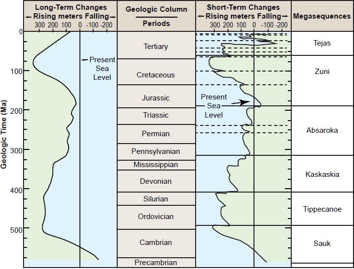
Fig. 1. Chart showing the secular timescale, presumed sea-level curve, and the six megasequences (modified from Snelling 2014a).

Megasequences Defined

Much of the Phanerozoic rock record has been divided into six sequences of deposition (Dapples, Krumbein, and Sloss 1948; Sloss 1963). Each sequence was defined as a discrete package of sedimentary rock bounded top and bottom by interregional unconformity surfaces across the North American craton (Sloss 1963). Oil and gas geologists working for Exxon further advanced the concept of sequences to include identifiable patterns on seismic data, creating seismic stratigraphy in the process (Payton 1977). Mitchum (1977) further defined each sequence as a stratigraphic unit of relatively conformable; genetically-related strata bounded top and bottom by unconformity surfaces.

Sequences supersede and include multiple geologic systems and in many instances can be recognized by their bounding erosional surfaces and sudden changes in rock type, independent of fossil content. Sequences record the sedimentology of the Flood, while fossils record what flora and fauna were buried within each sequence. They differ from the standard geologic timescale in that they are not based on changes of fossil content as are the Eras, Periods and Epochs (Fig. 1).

The terminology associated with sequence stratigraphy has ballooned in the past decades, causing some to use the term “megasequence” for the most prominent regional unconformities (Hubbard 1988). Haq, Hardenbol, and Vail (1988) then used the term “megasequence” to designate their First Order sequences, or their largest scale sequences, equivalent to Sloss sequences. Other secular and creation scientists have followed, using the term “megasequence” to describe rock-stratigraphic units traceable over vast areas bounded by unconformities (or their correlative conformities) (Davison 1995; McDonough et al. 2013; Reijers 2011; Thomson and Underhill 1999). Hereafter, this term will be used to designate the six, Sloss-defined megasequences.

The Creation of the Global Sea Level Curve and Megasequences

Vail et al. (1977) first identified global sea level (eustasy) as the dominant driving mechanism for megasequence development. Megasequences are thought to have formed as sea level repetitively rose and fell, resulting in flooding of the continents up to six times in the Phanerozoic (Sloss 1963). Upper erosional boundaries were created as each new sequence eroded the top of the earlier sequence as it advanced. The result was the first published global sea-level curves for the Phanerozoic.

Vail et al. (1977) and Haq, Hardenbol, and Vail (1988) used geohistory analysis and biostratigraphic data and paleo-environmental interpretations across selected continental margins to create and refine their global sea-level curves (Fig. 1). Their resultant curve shows the highest sea levels were reached in the Ordovician and in the Late Cretaceous. It is significant to note that Vail and Mitchum (1979) have acknowledged that their sea-level changes from the Cambrian through Early Triassic are not as well constrained as those from the Triassic upward. Little has been added to the details of the Early Paleozoic sea-level fluctuations which include the earliest three megasequences.

However, it should be noted that the secular sea-level curve is based on uniformitarian, environmental interpretations of many sedimentary units. For example, most secular geologists claim the Permian Coconino Sandstone was deposited on dry land, implying sea level was lower on the global curve during its deposition. In contrast, Whitmore et al. (2014) have demonstrated rather conclusively that the Coconino Sandstone was deposited under marine conditions. Therefore, sea level was likely much higher during its deposition (during the Absaroka megasequence) than what is shown on the sea-level curve (Fig. 1).

Megasequences Have Been Correlated Globally

Although Sloss (1963) initially defined his megasequences across only the interior of North America, oil industry geologists quickly extended these sequence boundaries to the offshore regions surrounding North America and to adjacent continents using well logs, seismic data, and outcrops (Hubbard 1988; Soares, Landim, and Fulfaro 1978) (Fig. 2). Using these data, oil industry geologists have tracked the megasequence boundaries from the craton to the ocean shelves on the basis of distinctive seismic reflection patterns (many due to abrupt truncations) as well as lithologic changes (xenoconformities, Halverson 2017) in oil well bores (using downhole well logs, biostratigraphic data, and cores) (Hubbard 1988; Van Wagoner et al. 1990). These same Sloss-megasequence boundaries were correlated to at least three other continents based on seismic data and oil well drilling results (Hubbard 1988; Sloss 1972; Soares, Landim, and Fulfaro 1978; Van Wagoner et al. 1990). In fact, nearly identical megasequence boundaries were identified and aligned to global tectonic events in North America, the Russian Platform, Brazil, and Africa (Soares, Landim, and Fulfaro 1978) (Fig. 2).

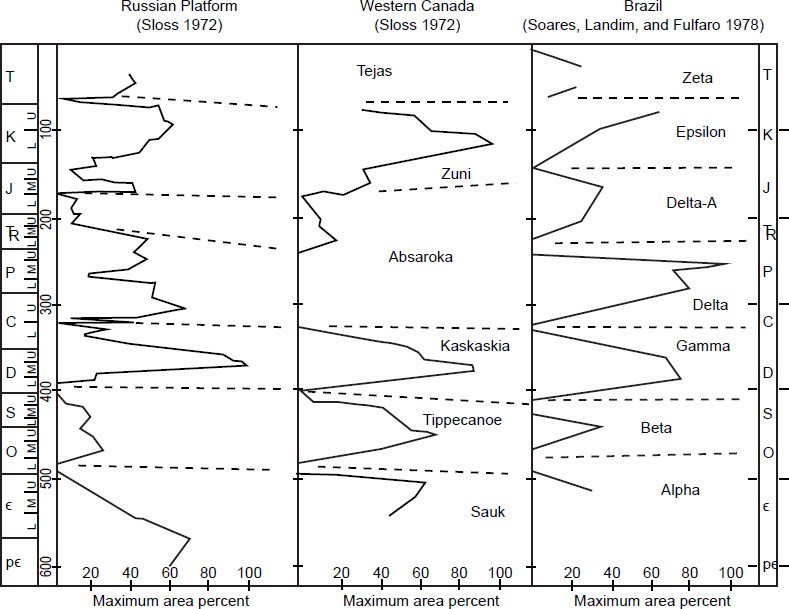
Fig. 2. Chart showing the correlation of megasequences across the Russian platform, Western Canada, and Brazil. Modified from Soares, Landim, and Fulfaro (1978). Note that Africa and South America were together as part of Gondwana up until the Zuni megasequence, and therefore likely share the same megasequence correlations.

Goal of This Investigation

Few researchers, if any, have attempted to map out the true extent of the sedimentological data and/or the volume of sedimentary rocks across the continents to verify the published results. This paper examines the rock record of the Flood sediments, megasequence-by-megasequence, mapping their extent across three continents. Conclusions are drawn based on the actual rocks that are observed in place. Particular attention is given to the Sauk megasequence which is generally assumed to be the first extensive layer deposited during the global Flood (Snelling 2014a).

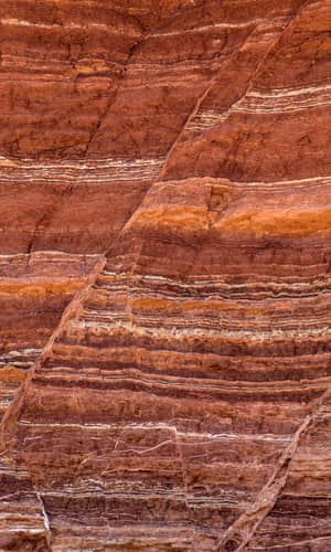
The continuity of the basal Sauk sandstone layer across the North American continent is a testimony to the extent and uniformity of the first great marine transgression of the Phanerozoic. In many places, the base of this layer is also known as the Great Unconformity (Peters and Gaines 2012). The basal Sauk megasequence is also coincident with the so-called Cambrian Explosion, where marine fossils representing many animal phyla suddenly appear in the rock record.

We recognize that there are locations that contain likely earlier Flood sediments below the Sauk level on a local scale, such as selected Late Proterozoic sediments in Grand Canyon of North America (Austin and Wise 1994).

Methods

Stratigraphic columns were compiled from published outcrop data, oil well boreholes, cores, cross-sections and/or seismic data tied to boreholes. Lithologic and stratigraphic interval data were input into a database, allowing thickness maps to be generated for the six, Sloss-defined megasequence intervals. These data were used to create a three-dimensional stratigraphic model across each of the three continents in this study. We also assumed the historical accuracy of the global Flood account as recorded in Genesis.

1. Collection of stratigraphic and lithologic data

Our database consisted of selected COSUNA (Correlation of Stratigraphic Units of North America) (Childs 1985; Salvador 1985) stratigraphic columns across the United States, stratigraphic data from the Geological Atlas of Western Canada Sedimentary Basin (Mossop and Shetsen 1994), and numerous well logs and hundreds of other available online sources. Using these data, we constructed 710 stratigraphic columns across North America, 429 across Africa, and 405 across South and Central America from the pre-Pleistocene, meter-by-meter, down to local basement. We recorded detailed lithologic data, megasequence boundaries, and latitude and longitude coordinates into RockWorks 17, a commercial software program for geologic data, available from RockWare, Inc. Golden, CO, USA. Fig. 3 is an example stratigraphic column from the Michigan Basin, showing the 16 types of lithology that were used for classification and the megasequences. Depths shown in all diagrams are in meters.

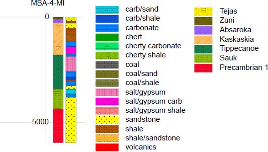
Fig. 3. Example stratigraphic column from the Michigan Basin illustrating the16 types of lithology that were used for classification and the six megasequences that were used in this study. Depth is in meters.

2. Creation of isopach maps

Sloss-type megasequence boundaries were identified within the stratigraphic columns across North America, South America and Africa. This paper examines primarily the Sauk megasequence and its intercontinental extent. Each continent was analyzed individually and isopach maps were constructed using the RockWorks 17 software that represented the entire Sauk megasequence. Figs. 4, 5, and 6 show the Sauk, Tippecanoe, and Kaskaskia isopach maps for North America, South America, and Africa, respectively.

3. Compilation of data by megasequence

RockWorks 17 allowed accurate summation of the total volume of each rock type by megasequence. Figs. 7, 8, and 9 show graphs of the volume of total rock in each megasequence by continent, broken down into six commonly observed rock types. We estimated our original “sand/shale” designation to be approximately 2/3 shale in order to determine a total sand and shale volume for each megasequence. All values shown are in cubic kilometers.

RockWorks 17 also allowed us to compile the total area covered by the Flood sediments across each continent. Table 1 shows the surface area covered, the volume of sediment, and the average thickness for each megesequence, continent by continent, and totaled, for the three continents in this study.

Results

According to Fig. 1, global sea level is supposed to have reached an extreme high in the Late Cambrian/Early Ordovician. The maximum level shown for the Sauk megasequence is about 300 m above the present ocean level. Secular geology textbooks commonly refer to the Ordovician as the “water world” because it is assumed that the ocean reached one of its highest levels during that time. However, data presented in this paper indicate the global sea level curve may not be as accurate in an absolute sense.

The areal extent of the Sauk megasequence across North America is quite impressive, covering over 12 million km² (Table 1 and Fig. 4). Sauk deposits are several kilometers thick along the east and west coasts of the North American continent. And yet, the Sauk is very thin (a few tens of meters) to non-existent across the central part of the continental USA. It averages only about 275 m across the North American continent where present (Table 1). Clarey (2015a; 2015b) described this thin zone across the central USA as possibly representing a pre-Flood lowland environment, flanked by shallow seas to the east and the west.

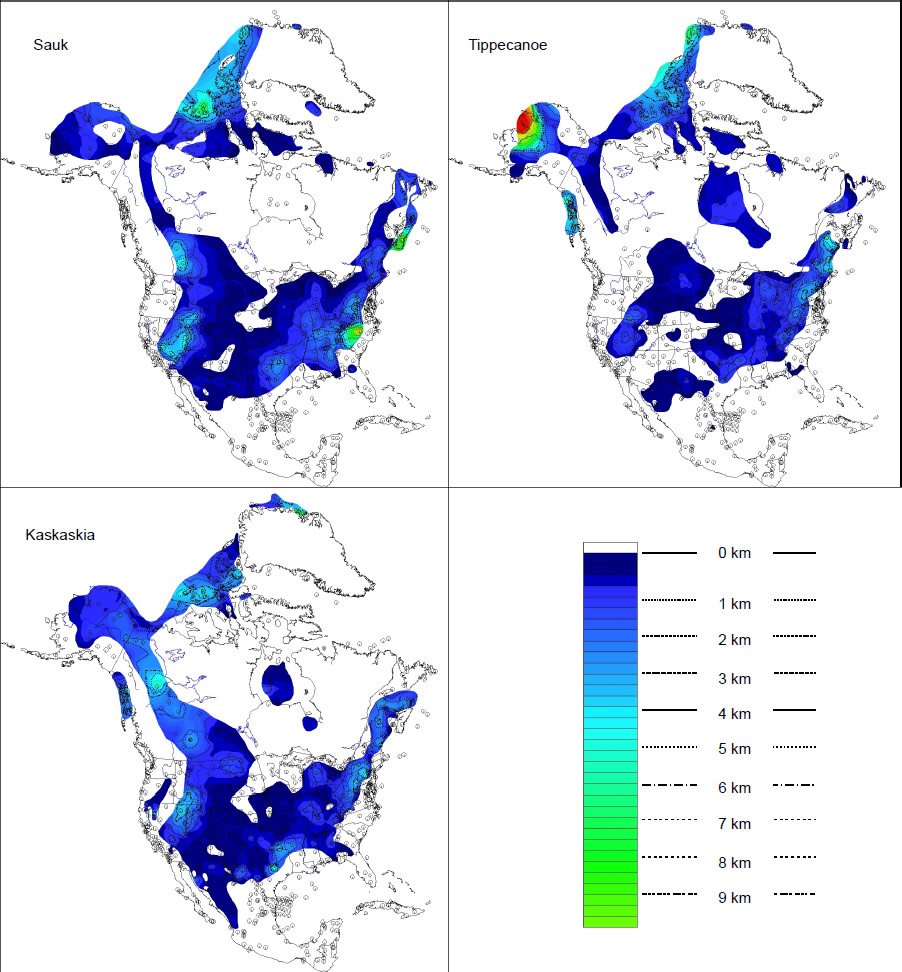
Fig. 4. Isopach maps of the Sauk, Tippecanoe, and Kaskaskia megasequences of North America. Scale is in kilometers.

In stark contrast to North America, the sedimentary rocks of the Sauk megasequence show very little extent across the South American (Fig. 5) and African continents (Fig. 6). The areal extent of the Sauk across South America is about 1.45 million km² and the areal extent across Africa is just under 9 million km² (Table 1). Both of these values are less than North America. In addition, only the northernmost part of Africa (beneath the Sahara) and the west-central portion of South America show Sauk sediments. Finally, the total volume of rock deposited during the Sauk represents the minimum amount for these three continents, compared to any other megasequence (Table 1).

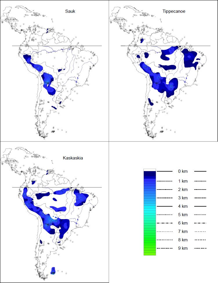
Fig. 5. Isopach maps of the Sauk, Tippecanoe and Kaskaskia megasequences of South America. Scale is in kilometers.

---

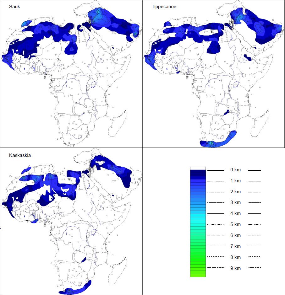
Fig. 6. Isopach maps of the Sauk, Tippecanoe and Kaskaskia megasequences of Africa. Scale is in kilometers.

Discussion

Can later erosion alone explain the patterns?

Fig. 7 shows the Sauk megasequence also has the least amount of total sedimentary volume preserved across North America, compared to all subsequent megasequences. Some of the total volumes shown in Fig. 7 have undoubtedly been reduced by later erosion, but exactly how much is uncertain. In spite of this uncertainty, it is likely the Sauk megasequence has preserved at least a reasonable proportion of the original volume deposited because we see consistent patterns in the surface coverage of the Sauk, Tippecanoe, and Kaskaskia megasequences on all three continents in this study (Figs. 7, 8, and 9 and Table 1). In fact, the Sauk, Tippecanoe, and Kaskaskia sequences (Lower Paleozoic) consistently demonstrate the lowest three preserved volumes of any of the megasequences on each continent and the thinnest average thicknesses also (Table 1).

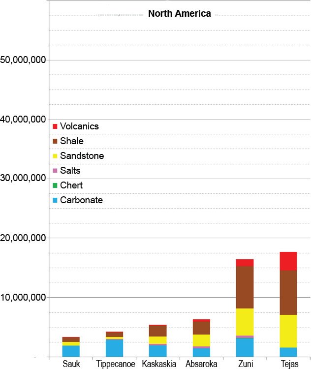
Fig. 7. Graph of the total volume of rock by megasequence for North America. All values are in cubic kilometers. The six major rock types are indicted by color.

Snelling (2014b), discussing the paper by Holt (1996), acknowledged that there is a disproportionate amount of Cretaceous (Zuni) and Tertiary (Tejas) sediment preserved in the rock record globally, compared to earlier deposits (Sauk through Absaroka, Fig. 1 and Table 1). However, Snelling (2014b) reasoned that it is impossible to know how much volume of the earlier megasequences may have been eroded and then were redeposited as Cretaceous and Tertiary strata. As a consequence, he concluded that higher amounts of later sedimentary strata should not be used as evidence for an Upper Cenozoic Flood/post-Flood boundary. Likewise, he reasoned that the limited amounts of Sauk, Tippecanoe, and Kaskaskia strata found across North America were likely greatly reduced by erosion during the receding phase of the Flood.

Admittedly, it is difficult to determine exactly how much erosion may have occurred if the material is now presumably missing. But, if there were lots of earlier erosion that reduced the volume of all pre-Cretaceous strata significantly, there should still be evidence to observe. Recall also, the small volume of Sauk found across North America (Fig. 7) is mimicked by a similarly small volume in the Tippecanoe and Kaskaskia megasequences. This relationship is further mimicked by the other two continents in this study which also show markedly less sediment volume in the first three megasequences compared to the later megasequences (Figs. 8 and 9).

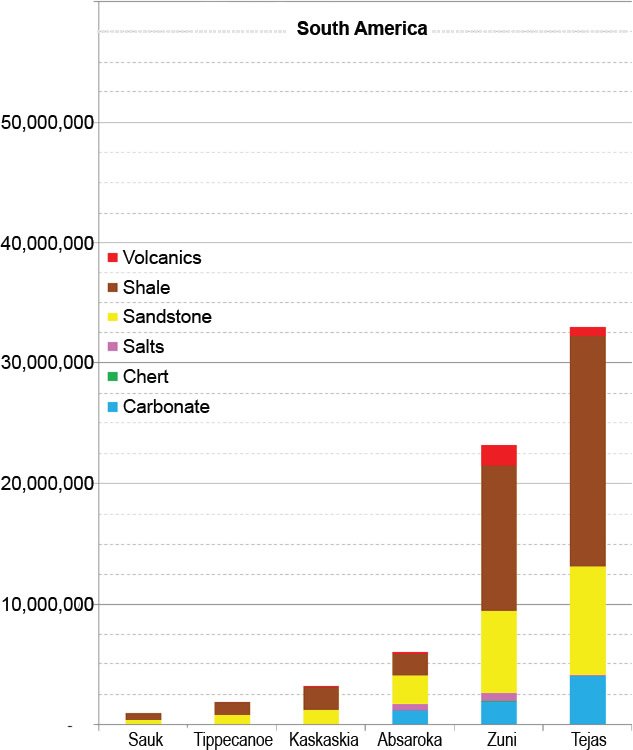
Fig. 8. Graph of the total volume of rock by megasequence for South America. All values are in cubic kilometers. The six rock types are indicated by color.

---

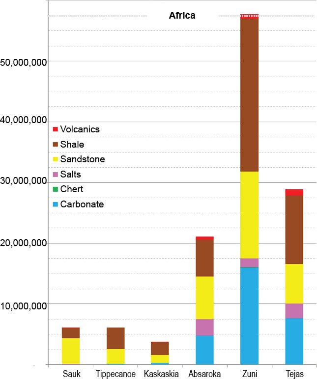
Fig. 9. Graph of the total volume of rock by megasequence for Africa. All values are in cubic kilometers. The six rock types are indicated by color.

However, the argument that all earlier strata were significantly reduced by erosion caused by mountain-building near the end of the Flood can be countered by several observations. First, the consistent internal stratigraphy of each megasequence testifies against significant erosion. Most megasequences start out with sandstone followed by shale and then carbonate. For example, the Sauk megasequence still exhibits a complete cycle consisting of basal sandstone (Tapeats equivalent), followed by shale (Bright Angel equivalent), and topped by a carbonate (Muav equivalent). This pattern is preserved in most of the earlier megasequences and in the Zuni and Tejas too. Vast erosion in between each megasequence cycle would have likely destroyed this systematic signature in many locations, if not totally. And yet we observe the entire sequence of sandstone, shale, and carbonate in the Sauk megasequence, not just the basal sandstone layer, across large portions of North America. This also explains the presence of so much carbonate and shale in the Sauk as shown on Fig. 7.

Secondly, we do not observe significant numbers of reworked fossils and mixed fossil debris in younger, Cretaceous and Cenozoic strata. Massive late Flood or post-Flood erosion should have transported vast amounts of fossil material and microfossils from the earlier megasequences, mixing them into younger sediments so that the fossil patterns would be less discernable in the later megasequences. This is not what is observed. The pattern of sudden appearance, stasis, and sudden disappearance of fossils is prevalent throughout the entire Phanerozoic sedimentological record, Sauk through Tejas (Wise 2017). Reworking significant amounts of fossils would likely have blurred this pattern.

Third, there was no large Cenozoic mountain-building event in Africa to erode and serve as a major source of Cenozoic sediment. North and South America have the Cenozoic-age Rocky Mountains and Andes Mountains, respectively. These two uplifts served as a major sediment source for the Tejas megasequence for these two continents. And yet we see the same pattern of very small volumes of Sauk through Kaskaskia, and tremendous amounts of Zuni and Tejas, across Africa just like we see on the other two continents. Why is Africa showing the same pattern of deposition if this is all the result of late Flood/post-Flood uplift and erosion of earlier megasequences?

We also observe consistency in the areal extent (surface area) of the early megasequences on each of the three continents (Table 1). This is particularly noticeable in South America and Africa and in the three continent totals (Figs. 5 and 6 and Table 1). If erosion did significantly reduce the thickness of earlier sediments, there should still be many small remnants of the Sauk through Kaskaskia scattered across the continents, and in randomly distributed patterns. We do not see this pattern. In fact, and even more compelling, is the observation that the early megasequences are confined to nearly the same identical sections of the same continents, and stack uniformly one on top of the other. This pattern is particularly noticeable across North Africa (Fig. 6) and to a slightly lesser extent, South America (Fig. 5). And even the more extensive areal coverage shown by the three earliest megasequences across North America is consistently marked by thinner deposits across the central USA (Clarey 2015a, 2015b) (Fig. 4).

Finally, the total surface areas covered by the first three megasequences across the three continents are nearly identical, varying only from 22.6 to 23.7 million km² (Table 1). All total surface areas increase greatly in the three subsequent megasequences (Absaroka–Tejas), with coverage varying from 35.6 to 56.9 million km² (Table 1). Also, the average sediment thickness totals for the three continents are nearly identical for the first three megasequences (Sauk–Kaskaskia) at about 500 m (Table 1). All later megasequences show much greater total average thicknesses (941 m–1712 m). Finally, the total sediment volume for the three continents for the first three megasequences (Sauk–Kaskaskia) only varies between 10.4 and 12.4 million km³ (Table 1). All subsequent megasequence total volumes increase significantly (33.5–97.4 million km³). The consistency in these total values alone makes a strong argument against significant erosion of the early megasequences.

The above patterns observed for each of the first three megasequences are not explainable as mere erosional coincidence. Instead, they are best explained by similar patterns of deposition across the same areas of the same continents. Erosion would not leave this consistent of a megasequence pattern on each of the three continents.

Erosion vs. nondeposition

Our study also found that all megasequences thinned toward the crystalline shield areas on all three continents. In other words, the stratigraphic units do not show evidence of massive erosion and truncation. Instead, they all thin in the direction of the now exposed shields, implying they were originally deposited thinly in these areas right from the start and are not a simple consequence of erosion. Fig. 10 shows four stratigraphic profiles across the northern USA. All show dramatic thinning of the megasequences from south to north toward the Canadian Shield, in support of this interpretation.

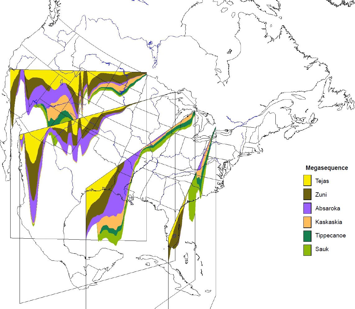
Fig. 10. South to north cross-sectional profiles showing thinning of megasequences in North America toward the Canadian Shield.

In addition, these four profiles (Fig. 10) show the improbability that erosion by the receding water (or post-Flood) phase of the Flood could serve as an explanation for the limited amounts of Sauk, Tippecanoe, and Kaskaskia we observe. Fig. 10 shows that the rocks of the Absaroka and Zuni megasequences cover and protect much of the earlier megasequences, preventing their late Flood or post-Flood erosion across much of North America (and the other two continents also). There was undoubtedly some erosion as each megasequence regressed and a new megasequence transgressed, but not a late or post-Flood erosional event as suggested to explain the high volumes for the Tejas (Snelling 2014b). Therefore, the simple argument that massive erosion can be used to explain the megasequence patterns we observe can be put to rest.

Is the global sea level curve accurate?

Most of these Lower Paleozoic strata are filled with marine fossils, implying that most of these early megasequences are exclusively marine in origin. If the global sea level rose to the level indicated in Fig. 1 there should be extensive deposits of Sauk strata across much of the earth. Where is the evidence of this flooding in the continental rock record? Why is there so little Sauk sediment preserved across Africa and North and South America? It appears that this lack of Sauk volume cannot be explained by mere erosion. The total surface area and total volume of sediment deposited during the Sauk, compared to subsequent megasequence cycles, strongly conflicts with the high sea level implied from Fig. 1. The collective results from each of the three continents are too consistent. It seems more likely that the global sea level curve is inaccurate in an absolute sense and that the ocean level during Sauk deposition never rose to the height necessary to have flooded much of the world’s continental masses. At least that is what the preserved rock data show.

Conclusion

If the Sauk megasequence truly represented one of the highest sea levels in global history (Fig. 1) there should be extensive deposits of Cambrian and Lower Ordovician rocks across all continents. However, that is not what is observed. Instead, the sedimentary rock record suggests that the Sauk megasequence probably represented only a minor rise in global sea level, compared to the later megasequences. Admittedly, it is also possible that sea level did rise higher during the Sauk transgression but left no deposits in some locations. However, the consistency of the thicknesses, volumes, and areal extent of the Sauk, Tippecanoe, and Kaskaskia megasequences, as pointed out in this paper, argue against this possibility. Furthermore, a higher Sauk sea level would have undoubtedly mixed in more terrestrial fossils in the first three megasequences. The record of predominantly shallow marine fossils in the first three megasequences therefore precludes significantly more extensive flooding than the rock record preserves. Finally, the likelihood of dominantly erosive processes leaving a nearly identical sedimentological signature across three continents, for three consecutive megasequences, is extremely improbable. Significant erosion would have most likely left more random patterns and little consistency, as is observed.

Indeed, data presented in this paper suggest the Floodwaters rose progressively as described in Genesis chapter 7. The consistently small volumes and thicknesses of Lower Paleozoic strata, and the consistent depositional locations of the first three megasequences, support the interpretation that only limited flooding occurred during the Sauk event. The Sauk megasequence likely was only part of a violent beginning to the Flood (during the first 40 Days), creating the Great Unconformity at its base and encasing prolific numbers of hard-shelled marine fossils, defining the Cambrian Explosion. The peak height of the Floodwaters (Day 150) seems to have occurred later, possibly during the Zuni megasequence, as that is when the volume of sediment also peaks on most of the continents (Figs. 7, 8, and 9 and Table 1).

We conclude that the published global sea-level curve is inaccurate in an absolute sense and should only be considered relative at best. The sedimentary record shows only a minimal sea-level rise occurred during the Sauk depositional event. In addition, the amount of pre-Flood dry land inundated during Sauk deposition seems to have also been limited. As suggested by Clarey (2015a, 2015b), the Sauk probably represents the effects of tsumani-like waves that transported sediment across pre-Flood shallow seas, and not across land masses. This could also possibly explain why so few, if any, terrestrial animals and plants are found as fossils in Sauk megasequence rocks.

References

Austin, S. A., and K. P. Wise. 1994. “The Pre-Flood/Flood Boundary: As Defined in Grand Canyon, Arizona and Eastern Mojave Desert, California.” In Proceedings of the Third International Conference on Creationism. Edited by R. E. Walsh, 37–47. Pittsburgh, Pennsylvania: Creation Science Fellowship.

Barrick, W. D., and R. Sigler. 2003. “Hebrew and Geologic Analyses of the Chronology and Parallelism of the Flood: Implications for Interpretation of the Geologic Record.” In Proceedings of the Fifth International Conference on Creationism. Edited by R. L. Levy, Jr., 397–408. Pittsburgh, Pennsylvania: Creation Science Fellowship.

Childs, O. E. 1985. “Correlation of Stratigraphic Units of North America-COSUNA.” American Association of Petroleum Geologists Bulletin 69 (2): 173–180.

Clarey, T. L. 2015a. “Examining the Floating Forest Hypothesis: A Geological Perspective.” Journal of Creation 29 (3): 50–55.

Clarey, T. 2015b. “Dinosaur Fossils in Late-Flood rocks.” Acts & Facts 44 (2). http://www.icr.org/article/dinosaur-fossils-late-flood-rocks.

Coffin, H. G. 1983. Origin by Design. Hagerstown, Maryland: Review and Herald Publishing Association.

Dapples, E. C., W. C. Krumbein, and L. L. Sloss. 1948. “Tectonic Control of Lithologic Associations.” American Association of Petroleum Geologists Bulletin 32 (10): 1924–1947.

Davison, G. E. 1995. “The Importance of Unconformity-Bounded Sequences in Flood Stratigraphy.” Creation Ex Nihilo Technical Journal 9 (2): 223–243.

Halverson, G. P. 2017. “Introducing the Xenoconformity.” Geology 45 (7): 671–672.

Haq, B. U., J. Hardenbol, and P. R. Vail. 1988. “Mesozoic and Cenozoic Chronostratigraphy and Cycles of Sea-Level Change.” In Sea-Level Changes: An Integrated Approach: SEPM Special Publication 42: 71–108.

Holt, R. D. 1996. “Evidence for a Late Cainozoic Flood/Post-Flood Boundary.” Creation Ex Nihilo Technical Journal 10 (1): 128–167.

Hubbard, R. J. 1988. “Age and Significance of Sequence Boundaries on Jurassic and Early Cretaceous Rifted Continental Margins.” American Association of Petroleum Geologists Bulletin 72 (1): 49–72.

McDonough, K-J., E. Bouanga, C. Pierard, B. Horn, P. Emmet, J. Gross, A. Danforth, N. Sterne, and J. Granath. 2013. “Wheeler-Transformed 2D Seismic Data Yield Fan Chronostratigraphy of Offshore Tanzania.” The Leading Edge 32 (2): 162–170.

Mitchum, R. M. 1977. “Seismic Stratigraphy and Global Changes of Sea Level, Part 1: Glossary of Terms used in Seismic Stratigraphy.” In Seismic Stratigraphy—Applications to Hydrocarbon Exploration. Edited by C. E. Payton, 51–52. Tulsa, Oklahoma: American Association of Petroleum Geologists Memoir 26.

Mossop, G. D., and I. Shetsen. 1994. Geological Atlas of the Western Canada Sedimentary Basin. Calgary, Alberta, Canada: Canadian Society of Petroleum Geologists and Alberta Research Council.

Payton, C. E. 1977. Ed. Seismic Stratigraphy—Applications to Hydrocarbon Exploration. Edited by C. E. Payton, 1–516. Tulsa, Oklahoma: American Association of Petroleum Geologists Memoir 26.

Peters, S. E., and R. R. Gaines. 2012. “Formation of the ‘Great Unconformity’ As a Trigger for the Cambrian Explosion.” Nature 484: 363–366.

Reijers, T. J. A. 2011. “Stratigraphy and Sedimentology of the Niger Delta.” Geologos 17 (3): 133–162.

Salvador, A. 1985. “Chronostratigraphic and Geochronometric Scales in COSUNA Stratigraphic Correlation Charts of the United States.” American Association of Petroleum Geologists Bulletin 69 (2): 181–189.

Sloss, L. L. 1963. “Sequences in the Cratonic Interior of North America.” Geological Society of America Bulletin 74 (2): 93–114.

Sloss, L. L. 1972. “Synchrony of Phanerozoic Sedimentary–Tectonic Events of the North American Craton and the Russian Platform.” Proceedings of the 24th International Geological Congress, Montreal, Section 6: 24–32.

Snelling, A. A. 2009. Earth’s Catastrophic Past: Geology, Creation and the Flood. Dallas, Texas: Institute for Creation Research.

Snelling, A. A. 2014a. “Geological Issues: Charting a Scheme for Correlating the Rock Layers with the Biblical Record.” In Grappling with the Chronology of the Genesis Flood: Navigating the Flow of Time in Biblical Narrative. Edited by S. W. Boyd and A. A. Snelling, 77–109. Green Forest, Arkansas: Master Books.

Snelling, A. A. 2014b. “Paleontological Issues: Deciphering the Fossil Record of the Flood and Its Aftermath.” In Grappling with the Chronology of the Genesis Flood: Navigating the Flow of Time in Biblical Narrative. Edited by S. W. Boyd and A. A. Snelling, 145–185. Green Forest, Arkansas: Master Books.

Soares, P. C., P. M. B. Landim, and V. J. Fulfaro. 1978. “Tectonic Cycles and Sedimentary Sequences in the Brazilian Intracratonic Basins.” Geological Society of America Bulletin 89 (2): 181–191.

Thomson, K., and J. R. Underhill. 1999. “Frontier Exploration in the South Atlantic: Structural Prospectivity in the North Falkland Basin.” American Association of Petroleum Geologists Bulletin 83 (5): 778–797.

Vail, P. R., R. M. Mitchum, R. G. Todd, J. M. Widmeir, S. Thompson, III, J. B. Sangree, J. N. Bubb, and W. G. Hatlelid. 1977. “Seismic Stratigraphy and Global Changes of Sea Level.” In Seismic Stratigraphy—Applications to Hydrocarbon Exploration. Edited by C. E. Payton, 49–212. Tulsa, Oklahoma: American Association of Petroleum Geologists Memoir 26.

Vail, P. R., and R. M. Mitchum. 1979. “Global Cycles of Relative Changes of Sea Level from Seismic Stratigraphy.” In Geological and Geophysical Investigations of Continental Margins. Edited by J. S. Watkins, L. Montadert, and P. W. Dickerson, 469–472. Tulsa, Oklahoma: American Association of Petroleum Geologists Memoir 29.

Van Wagoner, J. C., R. M. Mitchum, K. M. Campion, and V. D. Rahmanian. 1990. Siliciclastic Sequence Stratigraphy in Well Logs, Cores, and Outcrops: Concepts for High-Resolution Correction of Time and Facies. Tulsa, Oklahoma: American Association of Petroleum Geologists Methods in Exploration Series, No. 7.

Walker, T. 2011. “Charts of biblical geologic model.” http://biblicalgeology.net/images/stories/resources/geological_model_1.pdf.

Whitcomb, J. C., and H. M. Morris. 1961. The Genesis Flood: The Biblical Record and Its Scientific Implications. Philadelphia, Pennsylvania: The Presbyterian and Reformed Publishing Company.

Whitmore, J. H., R. Strom, S. Cheung, and P. A. Garner. 2014. “The Petrology of the Coconino Sandstone (Permian), Arizona, USA.” Answers Research Journal 7: 499–532. https://answersingenesis.org/geology/rock-layers/petrology-of-the-coconino-sandstone/.

Wise, K. P. 2017. “Step-Down Saltational Intrabaraminic Diversification.” Journal of Creation Theology and Science Series B: Life Sciences 7: 8–9.