A Simulation of the 8,000-year Bristlecone Pine Dendrochronology Using Post-Flood Virtual Trees

Jordan, Marshall

by Marshall Jordan Published on May 13, 2026

Answers Research Journal 19 (2026): 1–18.

PDF Download Cite This

The views expressed in this paper are those of the writer(s) and are not necessarily those of the ARJ Editor or Answers in Genesis.

Abstract

The bristlecone pine dendrochronology extends to 8,000 years before present based on tree-ring pattern matching of living and dead trees and counting back from the present, assuming one ring per year. But if the Flood buried the world’s trees in sediments, then there are no trees older than about 4,500 years, and chronology should not be any longer than that. Faced with this mystery, Christians may be tempted to doubt the veracity of the Genesis record. Some have claimed that multiple rings per year invalidate the dendrochronology because the 8,000 year dendrochronology is constructed assuming only one tree ring per year. Others have questioned the statistical significance of the tree-ring pattern matches but all the bristlecone pine tree-ring matching statistics are robust. These facts call for an evaluation of the primary assumption of dendrochronology, that matching tree-ring patterns prove two trees lived at the same time and experienced similar climate features. This paper challenges this assumption by a simulation where virtual post-Flood trees, all less than 4,500 years old, are used to construct an 8,000-year dendrochronology using the same methods employed in making the bristlecone pine dendrochronology. To achieve this result, disturbance patterns are introduced to the tree-ring patterns of those virtual trees growing within 1,500 years of the Flood, causing tree-ring patterns to match due to shared disturbance features rather than shared climate features, which falsely extends the chronology back beyond the date of the Flood. By itself, this simulation does not invalidate the bristlecone pine dendrochronology, but it does offer an alternative interpretation suggesting that the 8,000 years may be illusory. This alternative interpretation is consistent with the historical record of the Flood given in Genesis, encouraging Christians to trust the Bible.

Keywords: dendrochronology, Bristlecone Pine, tree rings, computer simulation, Flood, cross-dating statistics, uniformitarian assumptions

Introduction

The Methuselah Walk 8,000-year dendrochronology of bristlecone pines ( Pinus longaeva) stands as a monument to the advancing science of tree-ring dating (Ferguson 1979). But its length challenges the Genesis record of the global Flood which wiped the earth’s surface clean of all its trees about 4,500 years ago. The contradiction prompts one to speculate what error has allowed the scientists to construct such a hyper-long dendrochronology. The most obvious error is their neglect of the biblical record of the global Flood, a cataclysm that negates the uniformitarian assumptions underlying the construction of their dendrochronology. They assume that bristlecone pines have always grown under conditions like those that prevail today, and composite tree-ring series allow annual tree rings to be pattern-matched and counted back in time for 8,000 years. They have made two main assumptions:

There is one ring per year; and
When tree-ring patterns match, the trees lived at the same time for the years of overlap.

If the biblical record is true, one or both assumptions must fail as the dendrochronology is extended back in time.

In this paper these assumptions will be challenged with a simulation of virtual post-Flood trees that demonstrates how tree ring pattern matching may fail to document the historical record of when the trees lived. A post-Flood dendrochronology based on the demographics of the virtual trees is transformed into an 8,000-year dendrochronology using the standard methods of tree-ring pattern matching. The cause of this transformation is the inclusion of disturbance patterns in the tree rings of the virtual trees making their tree rings pattern-match for years when the trees were not growing simultaneously. We begin with the history of dendrochronology and its methods.

A Brief History of Twentieth-Century Dendrochronology

Data collection from bristlecone pines in the White Mountains of California began in the 1930s when Andrew Douglass (1929) and Edmund Schulman (1954) of the Laboratory of Tree-Ring Research at the University of Arizona measured tree ring widths from living and dead trees. They began to pattern match the ring width series into a dendrochronology that extended back in time ultimately to 8,000 years (Pearson et al. 2022). Since then, methods to ensure accurate tree-ring width series cross-matching have been developed and several more multi-millennial chronologies have been published including the German oaks (Becker 1993; Friedrich et al. 2004), Irish oaks (Pilcher et al 1984), and Finnish pines (Larsson and Larsson 2018), among others. These long chronologies were developed through the rigorous application of scientific methods and verified by careful statistical analysis so that the scientists who conducted this work claim that the multi-millennial chronologies provide an accurate historical record of past climate. There is no reason to doubt such a claim for chronologies extending back only two or three thousand years. But when they extend back beyond the date of the Flood, without any reference to that catastrophe and its effect on tree growth, these claims should be questioned.

At first, creation scientists committed to the study of all things in the light of Scripture were unconcerned with the progress of the science of dendrochronology. Then a very ancient bristlecone pine tree was discovered in the White Mountains, the Methuselah tree, which is said to be over 4,000 years old. This raised concern because creation scientists were all too familiar with the secular scientists’ use of uniformitarian assumptions that contradict the biblical record (Sanders 2018). It wasn’t long before the bristlecone pine dendrochronology was extended well beyond the Flood date by adding long-dead trees to the master chronology. This called for a response from those committed to a young-earth biblical chronology.

The challenge presented by long dendrochronology was accepted, and the battle was engaged by several scientists with a young-earth creationist worldview (Lammerts 1976; Brown 1968; Hebert, Snelling, and Clarey 2018; Snelling 2017; Sorensen 1976; Woodmorappe 2003a, 2003b, 2009, 2018). Initially, creationists argued that bristlecone pine tree rings were too thin to be accurately measured since many were thinner than human hairs (about 0.1 mm). Others argued that there could be multiple rings per year, and they could not simply be counted back in time. These objections have been answered by scientists who studied bristlecone pines although perhaps not to everyone’s satisfaction. They developed microscopic techniques to accurately measure the rings, and they asserted that bristlecone pines grow only one ring per year. In the 1970s, powerful statistical methods were developed to validate pattern matching of measured ring width series. Creationists had to hone their critique into a sharper instrument to probe this arcane science.

Recently creationist John Woodmorappe, after a careful and thorough review of the bristlecone pine dendrochronology statistics, developed the Migrating-Disturbance Hypothesis and the Disturbance-Clustering Hypothesis to explain how an 8,000-year-long dendrochronology could be constructed with post-Flood trees less than 4,500 years old (Woodmorappe 2003a). His main idea is that the post-Flood millennium was characterized by an unstable environment and an increased likelihood of random events causing disrupted growth of individual trees. According to this hypothesis, the primary uniformitarian assumption of tree-ring dating failed as the bristlecone pine dendrochronology was extended back in time by pattern matching the rings of dead trees. That uniformitarian assumption is simply this: the pattern matching of tree-ring series indicates the trees lived simultaneously and experienced the same environmental variables, and that their tree rings vary in width in like manner. That assumption fails if the disturbed ring patterns of two trees can match for rings in different years. Tree-ring dating depends on pattern matching which is based on several concepts that will now be reviewed.

Tree-Ring Dating Concepts

Tree-ring dating comes from an understanding of how trees grow. In temperate climates, trees produce annual rings because the tree is dormant in the winter and begins growing in the spring. Spring rains cause the outermost (cambium) layer of living cells under the bark to begin growing rapidly making large cells in the wood. This growth slows in the late summer forming smaller cells. Growth stops in the late fall completing the annual ring with a dark line of tiny cells (Sanders 2018). Since the tree grows only on the outermost ring, the inner rings are dead wood. These tree rings can be counted back in time on cores taken from living trees, and the dead wood of the inner rings can be sampled for radiocarbon content allowing construction of a radiocarbon calibration curve (Pearson et al. 2022; Reimer et al. 2020). The dendrochronology developed from the living trees can be extended back in time by matching tree rings from dead trees (called “subfossil trees”). These tree-ring patterns are like barcodes identifying the years that the trees were growing. The ring widths vary from year to year depending on environmental and climate variables such as regional rainfall, prevailing temperature, and cloud cover. For example, in wet years, the tree rings are fatter, and in dry years, the tree rings are thinner. This leads to trees that lived at the same time having ring widths that vary from year to year in the same manner (Miller and Cooper 1976). When the ring width patterns of two trees match, they are said to “cross-date.” This term implies that the series match because they lived together on the same dates. But since this paper challenges that assumption, the term “cross-match” will be used instead. Fig. 1 illustrates the cross-matching of tree-ring width patterns which will be called “ring width series” or “series” in what follows. The number of rings that are aligned is important. If the ring width series of two dead trees correlates over a suitably large number of rings, the two dead trees are thought to have lived at the same time. If the cross-matched ring width series is long enough to reach statistical significance, this is considered proof that the trees were both alive for those years.

The long bristlecone pine dendrochronology is based on the principles of tree-ring cross-matching described above. The 8,000-year length is incompatible with the historical record of Genesis, and the assumptions involved with constructing the dendrochronology are suspect. The problem is its excessive length in relation to the biblical chronology.

Several questions must be addressed: Is there only one tree ring per year, or can there be multiple rings? Were each of the cross-matches of the bristlecone pine subfossil trees statistically valid? Are shared climate features between trees the only cause for tree-ring patterns to match? After careful investigation, including fieldwork with bristlecone pines in the White Mountains, Woodmorappe was able to answer the first two questions in the affirmative. Yes, assuming one ring per year is generally correct today. And yes, the individual cross-matches in the bristlecone pine dendrochronology are statistically valid. The issues raised by these two questions did not overturn the bristlecone pine dendrochronology. But the third question could not be answered clearly. Therefore, in response to this, he proposed that environmental disturbances could cause ring width series to cross-match in a time-staggered manner meaning that the overlapping rings did not grow in the same years (Woodmorappe 2009).

The hypothesis is that tree ring series of dead trees can cross-match for two reasons: they shared the same climate, or they experienced similar disturbances. Both affect tree growth and determine how wide the tree rings are. Climate features often affect all trees living in the same area at the same time. They all experience the same rainfall and the same drought, the same sunlight and the same temperatures, causing their tree rings to be fat or thin in the same years. But a disturbance, such as a landslide or a flash flood, can affect one tree but spare its neighbors. For example, bristlecone pines in the White Mountains have thin root systems and grow on unstable rocky slopes. A boulder could be dislodged by rain or an earthquake, and running into one tree disrupt its root system so that the tree does not grow for several years before recovering from the injury. This would produce thin or absent rings in the injured tree but not in the neighboring trees. If two trees living at different times experienced a similar disruption, they could have similar ring width patterns induced by these disruptions. This could cause their series to cross-match in a “time-transgressive” manner. That is, the overlapping rings would not represent the same years, and the rings should not be counted as a span of years attached to the calendar. The bristlecone pine dendrochronology could be artificially long because subfossil trees growing in the first centuries after the Flood experienced an unstable environment with many disturbances affecting the growth of individual trees, and their tree-ring series would not form a valid dendrochronology.

This paper suggests a reinterpretation of the long bristlecone pine dendrochronology by demonstrating the disturbance hypotheses through a simulation on virtual post-Flood trees. It will show that tree-ring disturbance features could account for the extension of the bristlecone pine dendrochronology back in time beyond the date of the Flood even though all the bristlecone pine trees lived after the Flood. This simulation will be described in the Methods section after a review of the standard methods of dendrochronology.

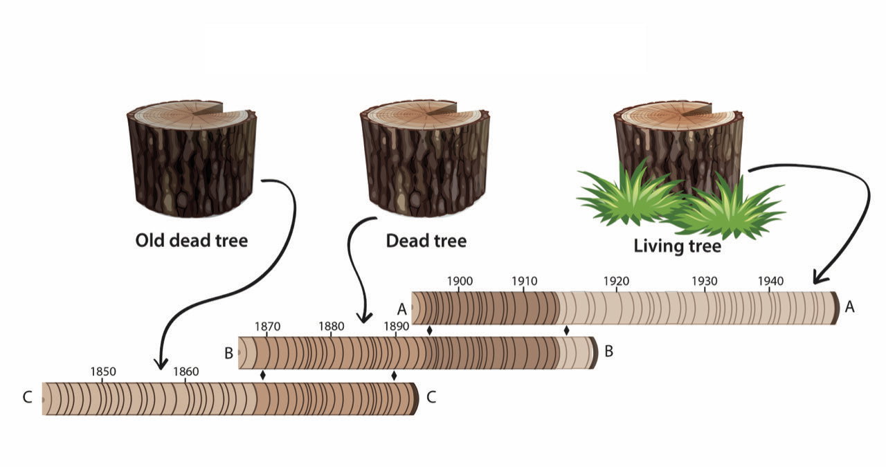
Fig. 1. Cross-matching of tree rings. An illustration of three tree-ring cores aligned with overlapping patterns for cross-matching. The youngest rings are closest to the bark on the right, and the oldest rings are closest to the pith on the left for each core. The B tree is older than the A tree, but the two were alive at the same time for a few years. Likewise, the C tree is older than the B tree, but the two were alive at the same time for a few years. Thus, the A rings partly overlap the B rings, and the B rings partly overlap the C rings allowing the ring counting and the time span to encompass the sprout age of the C tree to the death age of the A tree. If the A tree is still alive, then its outermost ring formed in the current year, and the absolute calendar dates of the rings in the three trees are known.

The Standard Methods of Tree-Ring Research

The study of tree rings proceeds in several phases:

Collection and processing of the cut surfaces or cores of trees to reveal the ring patterns.
Careful measurement of the tree-ring widths.
Cross-matching tree-ring width series among trees with overlapping life spans so that the rings can be counted back in time to make a dendrochronology.
If the dendrochronology can be anchored to the calendar, radiocarbon calibration curves can be made by measuring the ¹⁴C content of the tree rings.
A historical record of climate changes can be discerned in the dendrochronology.

Of these phases, this paper is concerned only with the cross-matching of tree-ring series and the construction of the dated dendrochronology by counting tree rings back in time.

Generally, the rings of a tree are assumed to represent the growth of individual years (Ferguson 1969; Ricker et al. 2020). For living trees, the outermost ring grew in the current year, and the inner rings can be counted back in time to the pith which represents the date the tree sprouted. The goal is to obtain the ring width series of older trees and by cross-matching, attach them to the growing chronology extending it further back in time. When no more living old trees are available, then the ring width series from nearby dead trees can be connected to the chronology by cross-matching. The concept is illustrated in fig. 1 where three tree cores are aligned in an overlapping fashion. The actual cross-matching is done on ring-width series which are lists of the tree-ring widths obtained by measuring the individual rings (Pearson et al. 2022).

The calendar-anchored dendrochronology made from living trees is extended into the past by cross-matching with tree-ring series from subfossil trees. These are long-dead but not fully fossilized trees found in the gravels along rivers, buried in peat bogs, or, in the case of the bristlecone pines, lying on mountain sides (Friedrich et al. 2004). In this manner, the bristlecone pine dendrochronology has been extended back to 8,000 years before present (BP).

For several reasons, cross-matching subfossil trees is difficult. One problem is that there is no guarantee that two dead trees found next to each other were growing next to each other in life. Dead trees may be blown over and roll down into a valley coming to lie next to other dead trees of a much different age. Since cross-matching of tree-ring patterns is often difficult even for live trees growing in the same area, one can understand the difficulty of cross-matching these subfossil trees. Sometimes the ring series of one subfossil tree cannot be cross-matched with any of the others because the rings are too thin to measure or too uniform in width. These series are called “complacent.” Complacent series cannot contribute to the dendrochronology (Ricker et al. 2020). The subfossil trees whose ring series are used to extend the chronology are carefully chosen from the available specimens and then submitted to the technique of cross-matching.

The raw data consists of a series of tree ring widths measured on a core boring or cut slab of a tree. The series is subjected to a mathematical normalization (Larson 2021). The normalized series are then compared in a stepwise fashion, and each alignment is scored for ring width correlation until the best match is identified.

Statistical and Mathematical Methods of Cross-Matching Tree Rings

The first step is to “normalize” (“standardize” or “detrend”) the ring width series for each tree to remove systematic bias caused by non-climactic factors that affect tree-ring growth patterns. These included geometric bias where larger diameter trees have thinner rings than smaller trees, and age bias where younger trees grow faster than older (Ferguson 1969; McPartland et al. 2020). This first step is necessary because a statistically valid cross-match is impossible unless the tree-ring width series are normalized to remove these biases.

Several formulae for normalizing the tree-ring series have been developed. The computer simulation presented will use the Baillie-Pilcher normalization method of eq. 1 (Baillie and Pilcher 1973; Keenan 2006)). Here, Norm(w_i)is the normalized i^th ring in the series, where the i^th ring has width w_i. To normalize w _i, it is divided by the mean of the widths of the five rings of which w_i is the center ring. Then the log is taken.

N o r m (w_{i}) = l o g (\frac{5 w_{i}}{(w_{i - 2} + w_{i - 1} + w_{i} + w_{i + 1} + w_{i + 2})})

(eq. 1)

The next step is to incrementally compare and score the normalized ring width series of two trees to determine the best cross-match. The theory of correlating tree-ring series to find the best cross-match is simple. If the ring widths of one tree are a set of values, x, and those of the other tree are a set of values, y, then x and y are “correlated” if they form a line when plotted as Cartesian coordinates. If x and y increase and decrease together, then they are positively correlated, and if they vary in opposite directions, they are negatively correlated. In the process of cross-matching two tree ring series, the degree of correlation is estimated for all overlaps of the series (Baillie and Pilcher 1973).

Here are the steps in the Baillie-Pilcher method. The normalized ring width series of the first tree is lined up with its youngest rings juxtaposed to the oldest rings of the second tree. Overlaps should begin at 50 rings because a cross-match made with fewer rings is considered insignificant. Dendrochronologists are reluctant to say exactly how many overlapping rings are needed, with many citing 60 or more, while admitting that they sometimes accept fewer (Bernabei and Franceschi 2025). The measured ring widths of the two tree-ring series are then compared by computing a Pearson correlation coefficient (PCC) and a student’s t-test based on the PCC and the number of rings overlapping. The process is then repeated after shifting by one ring to make a new alignment. At each alignment, the correlation and the t-value are recalculated. These well-known statistical tools (PCC and t-test) are now described as they are applied in cross-matching tree-ring series.

For each alignment of the two series, a PCC is calculated for the overlapping normalized ring widths using eq. 2, where x_i and y_i are the normalized widths of the aligned rings, x̄ and ȳ are the mean widths of the two series, and n is the number of overlapping rings.

PCC = \frac{(\sum_{i}^{n} (x_{i} - \bar{x}) (y_{i} - \bar{y}))}{{(\sum_{i}^{n} (x_{i} - \bar{x}) {}^{2}{\sum_{i}^{n}} (y_{i} - \bar{y}) \overset{2}{})}^{1 / 2}}

(eq. 2)

Then the PCC and overlap ( n) are used in eq. 3 to calculate the t-value. Because this t-value is calculated for series normalized by the Baillie-Pilcher normalization method, it is called the Baillie-Pilcher T Value (BPTV). Then the y series is stepped one ring at a time to the right against the x series, and the PCC and BPTV are calculated again for each step. In this way the two series are compared for all possible overlaps of 50 rings or more. The highest BPTV and its PCC and overlap are the best cross-match of the two series. The higher the BPTV, the better the cross-match.

It is a matter of opinion how high a BPTV must be to be significant. All agree that the scores below five are considered statistically weak. Confidence that a good cross-match has been found requires a BPTV of five or above (Keenan 2006). Therefore, in the simulation described below, a BPTV at or above five is considered significant. What is hoped for is a cross-match with BPTV much higher due to a higher PCC and longer overlap, and there will be no question that the cross-match is statistically significant.

t - value = \frac{PCC {(n - 2)}^{1 / 2}}{{(1 - {PCC}^{2})}^{1 / 2}}

(eq. 3)

When forming a dendrochronology, not all the subfossil trees need to be cross-matched but just those that are thought to be contemporaneous. The trees are arranged in groups based on ¹⁴C content, and then the trees in each group are cross-matched. This process is repeated until all the trees in the group are compared to one another. The best cross-matches are used for making the chronology. This chronology is “floating” relative to the calendar because an absolute date has not been determined for any of the rings which have not been counted back in time from the present or from any known calendar date. The final steps in completing the long dendrochronology is to join each group by cross-matching with the other groups. Finally, the composite series is joined to a historic dendrochronology that has been anchored to absolute calendar dates to everyone’s satisfaction. Dendrochronology is anchored to the calendar by cross-matching the tree-ring series to published dendrochronology that began with living trees whose outermost rings have a known calendar date. Theoretically, if enough subfossil trees are found and adequate cross-matching between the floating series can be achieved the dendrochronology is completed extending the historical record further back in time. This approach was successful in the case of the bristlecone pine dendrochronology where all the trees cross-match with robust statistics. Furthermore, there is reciprocity in that multiple trees above and below their final position in the chronology cross-match with strong statistics.

From the several correlation methods that have been devised, the Baillie-Pilcher T-value method described above was chosen for the simulation presented here (Baillie and Pilcher 1973). As will be described below in the results, both the Baillie-Pilcher and the CDendro normalization methods were used to verify the statistics for the bristlecone pine dendrochronology, so the two methods could be compared. The CDendro normalization divides the ring width for a given year by the sum of ring widths of that year and the next (Larsen 2021). The Baillie-Pilcher and the CDendro normalizations generally gave the same t-values for cross-matching tree-ring series and when they differed, the CDendro t-values tended to be slightly higher. Their performance being judged as equal, the Baillie-Pilcher normalization method was used to analyze the virtual dendrochronology because it is the more common method in the dendrochronology literature.

Methods

On November 6, 2025, the Graybill Methuselah Walk Bristlecone Pine data (GMW data file) was downloaded from the National Centers for Environmental Information website of the National Oceanic and Atmospheric Administration (https://www.ncei.noaa.gov/products/paleoclimatology/tree-ring). The 7,980 rows and 286 columns of this rectangular data file contain the tree-ring widths and the years of each tree ring for the 285 trees in the bristlecone pine dendrochronology. There are 7,979 rows for the years and 285 columns for the trees whose names head the columns. Python scripts, described in the next section, were written to extract relevant information for plotting and analyzing the dendrochronology. The Baillie-Pilcher statistics, that is, the series overlap, the Pearson correlation, and the Baillie-Pilcher t-value (BPTV), were generated for each pair of trees according to their arrangement in the dendrochronology. Then all 285 trees were cross-matched in pairs at all overlaps at or above 50 rings against all the other trees.

Computing Cross-match Statistics for the Bristlecone Pine Trees

A Python algorithm was made to compute the cross-match statistics of tree-ring series using the Baillie-Pilcher method described above. The algorithm proceeds with the following steps. First, the tree-ring width series of two samples was taken from the GMW data file, and the zero-width rings were replaced with a width of 0.01 mm. Each series was then normalized according to eq. 1. Next, the series were aligned one above the other with the first 50 rings of the top series juxtaposed to the last 50 rings of the lower. The two subsets were then correlated with eq. 2, and a t-value (the BPTV) was computed with eq. 3. The results (the overlap length, the PCC, and the BPTV) were recorded in a temporary file. The lower series was then stepped one ring to the right, the statistics were recalculated, and the results were recorded in the temporary file. This process was repeated until all possible alignments of the two series equal to or greater than 50 rings were analyzed and recorded. Finally, in a permanent file all cross-matches with BPTV equal to or greater than 5.0 were recorded for each pair of series. Since there were 285 trees in the GMW data file, this amounted to 40,470 pairs of series analyzed.

To determine the likelihood of finding a BPTV of 5.0 or greater by chance alone, the above algorithm was used to cross-match pairs of random ring-width series of 1,000 rings with the statistics computed for each alignment of 50 rings or more. The process of assigning random ring widths between 0.01 and 7.0 mm to two 1,000-ring series was repeated 100,000 times, and the number of BPTV equal to or greater than 5.0 was recorded for each iteration. This test of 100,000 iterations worked as a quality control to verify that the Python algorithm functioned correctly and to determine the likelihood that a BPTV of 5.0 could be produced by chance alone.

Summary statistics were calculated using the algorithm for each consecutive pair of trees in the bristlecone pine dendrochronology. The equal-length series of overlapping ring widths for each pair was extracted from the GMW data file, and the series were cross-matched. This same algorithm was incorporated into the pipeline used to analyze the virtual post-Flood trees which were made according to the method described below.

Constructing the Virtual Post-Flood Trees

The simulation consisted of a Python script “pipeline” available in Supplementary file 1 that proceeded in five phases.

Virtual post-Flood trees all less than 4,500 years old were made by randomly selecting sprout and death dates for each virtual tree. The number of tree rings was equal to the death date minus the sprout date assuming one tree ring per year.
Tree-ring widths were assigned to each tree ring in each virtual tree according to the method described below.
All the virtual trees were arranged in their true order of their demographics, and the ring width series were aligned exactly according to the years that the rings “grew.”
The Baillie-Pilcher statistics (BPTV) were calculated and recorded. These 4 phases are illustrated in fig. 2. When all the virtual trees were constructed, the dendrochronology was plotted based on the demographics of the trees. The data file containing the virtual trees used for illustration in this paper is available in Supplementary file 2.
After disturbance patterns (described below) were introduced into the virtual tree ring series, the dendrochronology was reconstructed based on cross-matching the virtual trees in their true order in the dendrochronology at all overlaps equal to or above 50 rings. The cross-matches with the highest BPTV were used to reconstruct the dendrochronology. For each run of the simulation, all phases of the simulation were repeated. Note that for each run of the simulation, two chronologies were made: one based solely on demographics and the other, the reconstruction, based on cross-matching virtual trees to which disturbance patterns had been added to the tree ring series. The phases will now be described in more detail.

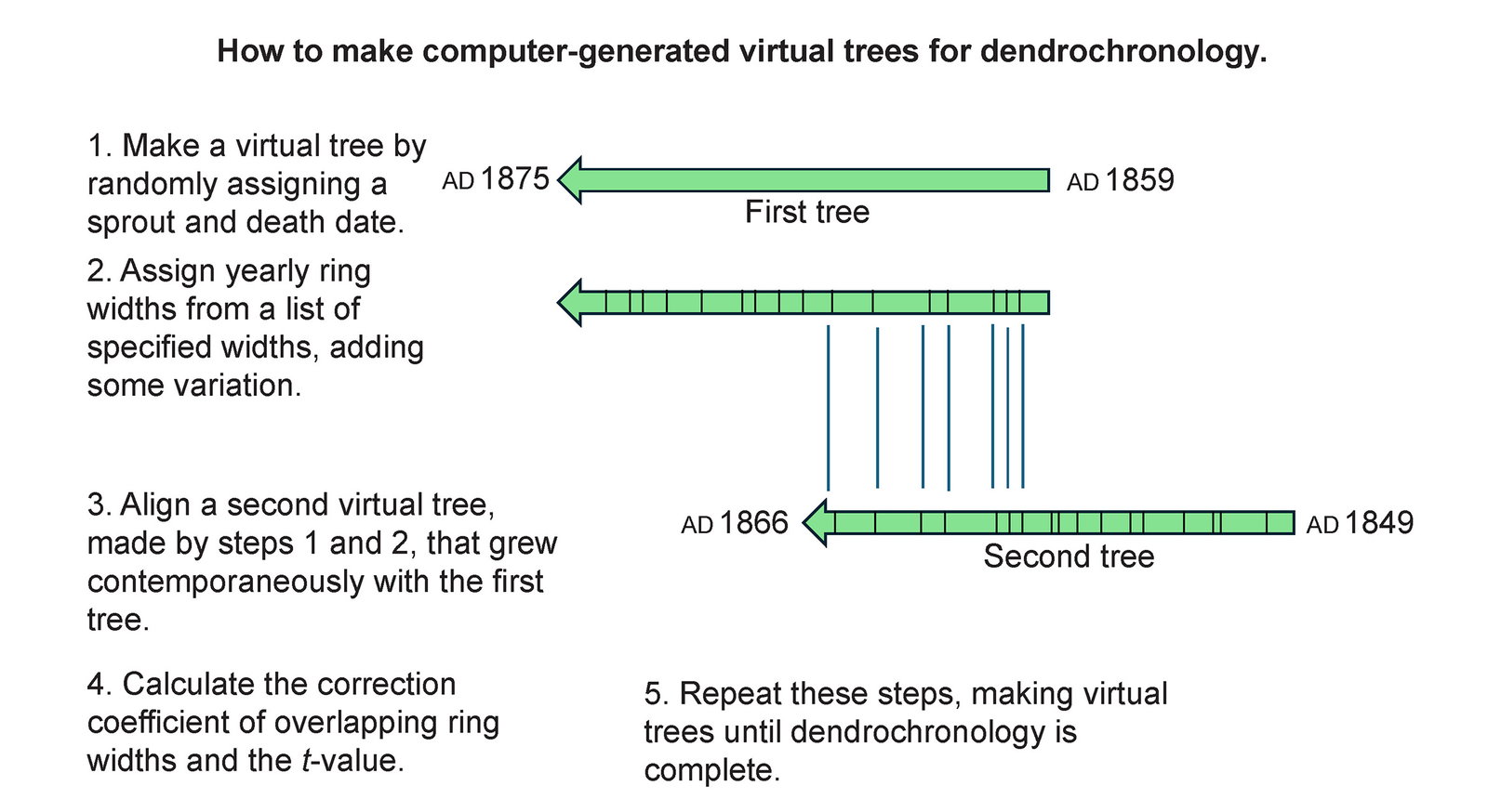
Fig. 2. An illustration of how the Python pipeline forms virtual trees. The tree-ring widths are assigned from a list of base-ring widths for each calendar year that are varied up or down by multiplying the base-ring width by ±0.5.

Since the bristlecone pine dendrochronology had 285 trees, the simulation generated 285 virtual trees with each run. These virtual trees were made by randomly assigning a sprout date and a death date within the 4,500 year post-Flood era for each tree. The number of rings was the difference between these two dates assuming one ring per year. The name of each virtual tree included the sample number and the sprout and death dates. Trees varied in life span from 500 to 2,000 years for the first (the recent) half of the chronology, and from 300 to 1,200 years for the second half because in the bristlecone pine dendrochronolog the oldest trees were not as long-lived as the youngest. The 30 youngest trees were assigned death dates of 0 years BP, indicating that they were still living trees. None of the randomly assigned sprout dates were allowed to be older than 4,500 years BP since that was the assumed date of the Flood. Thus, there were about 50 of the oldest trees that sprouted at the end of the Flood year. Next, ring widths were assigned for each of the 285 trees in one of two ways.

The first way of assigning tree-ring widths was based on a “climate signal” designed to account for shared environmental factors affecting tree growth for trees living at the same time. The climate signal was a list of 4,500 random numbers between 0.01 and 0.7. Each number was the base size in millimeters of the ring width for that year from the present at year 1, to the Flood at year 4500 BP. The climate signal tree ring widths for each tree were made by taking the base ring width of the corresponding year from this list and increasing or decreasing it and multiplying it by a factor randomly chosen between –0.5 and 0.5. The median variation by this method was zero. Varying the base ring width in this manner provided a semblance of life to the ring widths accounting for variations in soil and slope characteristics that affect the growth of real trees. Ring width series made using this method had a strong climate signal which gave robust statistical cross-matches when properly aligned.

For virtual trees living within 1,500 years of the Flood (between 4500 and 3000 BP), ring widths were also assigned according to the climate signal except that the strength of the climate signal was cut in half for every fifth and sixth tree. This was accomplished by replacing the ring widths of the climate signal for every even year with a random value between 0.01 and 0.7, so that every other ring had a random width. A disturbance pattern described below was then introduced randomly at two positions in each series. Thus, these older virtual trees had a weak climate signal and a disturbed ring width series. This alteration for the older virtual trees was in keeping with the hypothesis that the post-Flood 1,500 years were characterized by an unstable environment and an increased likelihood of random events disrupting individual trees. The disturbance pattern in the virtual trees older than 3000 BP consisted of placing a very narrow ring of 0.01 mm every five years and seven years for 30 occurrences. Because these disturbance patterns were randomly placed without reference to the date, they were “time transgressive,” that is, they allowed the series to cross-match for overlapping rings that were not simultaneous.

Forming the Simulation Chronologies

For each run of the simulation, two chronologies were made and plotted from the virtual trees, and cross-match statistics were computed. The first chronology (the virtual dendrochronology) and statistics were based on the demographics of the virtual trees. This was a perfect dendrochronology since the dates that the trees lived were known, and the contemporaneous overlaps of the series between any two trees were known. The second chronology (the disturbance dendrochronology) and associated cross-match statistics were based on cross-matching the series using the above-described Baillie-Pilcher algorithm. Consecutive pairs of series were lined up, and the statistics were calculated. The series were then shifted by one ring, and the statistics were calculated again. In this manner all possible combinations of the two series with overlaps above 50 rings were tested, and the alignment with the highest BPTV was chosen to place the series in the developing disturbance dendrochronology.

The Python scripts and supplementary files are available at the end of this paper with links.

Results

Fig. 3 is a plot of the bristlecone pine dendrochronology based on the tree ring width data from the GMW data file in Supplementary file 3. Each blue line is one of the 285 trees. The length of the line and its location relative to the horizontal axis represent the years of the tree’s life as assigned in the dendrochronology. The length of each tree’s life equals the number of tree rings. The 48 trees living in the present all bump up against the left vertical axis. Nine trees appear to have sprout dates at 8000 BP on the right of the horizontal axis, suggesting that these series had been truncated at this point. The pattern of this plot is thinner in the middle and fatter at either end because fewer of the 285 trees comprise the middle portion of the chronology between 2000 and 6000 BP, that is, from the third to the sixth millennia of the eight millennia long chronology. The lifespans of the trees and the lengths of their corresponding series vary from 124 years to 2,983 years. Fifty-five trees lived for over 1,000 years. The average tree lifespan was 747 years with a standard deviation of 476 years.

A BPTV value of 5.0 was determined to be the threshold for a statistically significant correlation by cross-matching 100,000 pairs of 1,000-ring series of random ring widths. All alignments above 50 rings were tested. By chance alone, pairs of random 1,000-ring series were found to have an alignment (of more than 50 rings) that cross-matched with BPTV of 5.0 or higher 3% of the time. In the 100,000 iterations, a BPTV equal to or greater than 6.0 and 7.0 occurred 0.5% and 0.04% of the time, respectively. The highest BPTV for these random series was 8.1.

The algorithm was then used to cross-match all possible pairs of the 285 Bristlecone pine trees. 33,031 of these 40,470 cross-matches were between non-contemporaneous tree pairs according to their demographics extracted from the GMW data file. The number of non-contemporaneous tree pairs that cross-matched with a BPTV equal to or greater than 5.0 was 7,448 or 23%. One pair of non-contemporaneous trees (MWK551 and MWK462) cross-matched with a BPTV of 13.0, but in only 14 cases were cross-matches at 10.0 or higher (0.0004%). One pair (MWK231 and MWK742) had these ten significant cross-matches: 6.1, 5.7, 5.7, 5.6, 5.4, 5.4, 5.3, 5.2, 5.1, 5.0.

The number of contemporaneous tree pairs that had more than one significant cross-match was 1,025 or 14%. Among these contemporaneous tree pairs, one pair (MWK632 and MWK631) gave the following 13 significant cross-matches: 25.7, 25.6, 25.1, 25.1, 20.7, 19.7, 18.8, 13.1, 12.1, 10.9, 7.2, and 6.5. Supplementary file 4 shows the results of the 40,470 cross-matches of all 285 trees against each other. The file has three columns. The first two columns display the two trees being cross-matched. The third column is a list of the significant Baillie-Pilcher t values, those equal to or greater than 5.0. When the list is empty, it means there were no significant cross-matches. All cross-matches with BPTV equal to or greater than 5.0 are listed. Since this file (Supplementary file 4) was made by testing all alignments of 50 rings or more, for comparison, the 40,470 cross-matches were repeated this time testing all alignments of one hundred rings or more (Supplementary file 5) which resulted in about 9% fewer significant cross-matches (Supplementary file 5).

Supplementary file 6 gives the statistics for the correlation of consecutive pairs of ring width series in the bristlecone pine dendrochronology (Supplementary file 6). This file contains seven columns. The first two columns list the trees being cross-matched. Column 3 (OVL) is the number of overlapping tree rings in the cross-match. Column 4 (PCC) is the Pearson Correlation Coefficient. Column 5 ( t-test) is student’s t-test. Column 6 (CDen) is the CDendro t-value. Column 7 (BPTV) is the Baillie-Pilcher t-value. Comparing the BPTV to the CDen results, one can see that they generally agree. These series were correlated at only one alignment, that recorded in the raw data file for the years the two trees lived simultaneously. Summary statistics for overlap, Pearson correlation, and BPTV are given in table 1, in the column labeled “Bristlecone Pine.”

Many of the trees in the bristlecone pine dendrochronology have rings with a width of 0.0 indicating that the tree ring for that year was missing. The number of missing rings in each tree of the bristlecone pine dendrochronology is in Supplementary file 7, and the number of missing rings per year is in Supplementary file 8.

Statistic	Bristlecone Pine	Virtual	Disturbance
Overlap mean	555	761	751
Overlap s.d.	330	355	362
Overlap range	112–2042	203–1970	157–1070
PCC mean	0.6671	0.5697	0.6911
PCC s.d.	0.1029	0.3834	0.2245
PCC range	0.4221–0.9926	–0.4143–0.9342	0.2682–0.9261
BPTV mean	21.9	33	35.8
BPTV s.d.	10.65	27.36	23.64
BPTV range	5.9–64.0	–8.1–84.9	6.3–84.9

Table 1. Summary statistics for the bristlecone pine, virtual, and disturbance dendrochronologies. The bristlecone pine statistics are from cross-matching consecutive pairs of trees based on their demographics (sprout and death dates) in the Graybill Methuselah Walk data file. The virtual dendrochronology statistics are from cross-matching consecutive trees in the post-Flood virtual trees based on their demographics. The disturbance dendrochronology statistics are from cross-matching consecutive tree pairs of the virtual dendrochronology at all possible overlaps simulating the methods of standard dendrochronology construction

To discern differences in tree growth between the oldest and youngest trees in the bristlecone pine dendrochronology, the average tree-ring widths for the first 200 years of life were computed for trees living in the first millennium and last millennium of the chronology. These are illustrated in fig. 4. The average tree ring size for the first 200 years of life for trees living in 7000–8000 BP (6000–5000 BC) is 0.27. The average tree ring size for the first 200 years of life for trees living in 1000–0 BP (AD 979–1979) is 0.22. Thus, the rings of ancient trees are 20% larger than those of modern trees.

Fig. 5 is the perfect virtual dendrochronology of one characteristic run of the simulation. This perfect dendrochronology is based on demographics and the sprout and death dates of the post-Flood virtual trees. The practice of dendrochronology would be a trivial pursuit indeed if real subfossil trees, like virtual trees, came labelled with their sprout and death dates. But real-world subfossil trees must be cross-matched to find out, if possible, when they lived. The statistics for the correlations of consecutive pairs of trees in this perfect virtual dendrochronology are given in Supplementary file 9. Summary statistics for overlap, PCC, and BPTV are given in table 1.

Fig. 6 is the disturbance dendrochronology constructed by cross-matching all possible alignments of the consecutive pairs of virtual tree ring series using the standard methods of dendrochronology. The younger virtual trees formed the same pattern matches as in the first perfect dendrochronology due to the strong climate signal and the absence of any disturbance to the ring widths. Due to the weak climate signal and the disturbance patterns, the series for the older virtual trees cross-matched to form a longer dendrochronology. Each run of the simulation gives a different result, and fig. 6 shows one particular run of the simulation. Each run gives the illusion of a different extent back in time due to the stochastic elements of the simulation. No two runs are identical. The simulation was adjusted so that on average the disturbance dendrochronology seems to extend back to about 8000 BP. This means the simulation was tuned to model the bristlecone pine dendrochronology. Fig. 7 shows both the virtual dendrochronology and the disturbance dendrochronology on the same plot. Fig. 8 shows the results of 24 runs of the simulation where each line is made from the death dates of the virtual trees as determined by their cross-matching in the chronology. The statistics for the consecutive series in the disturbance dendrochronology run shown in fig. 6 are given in Supplementary file 10.

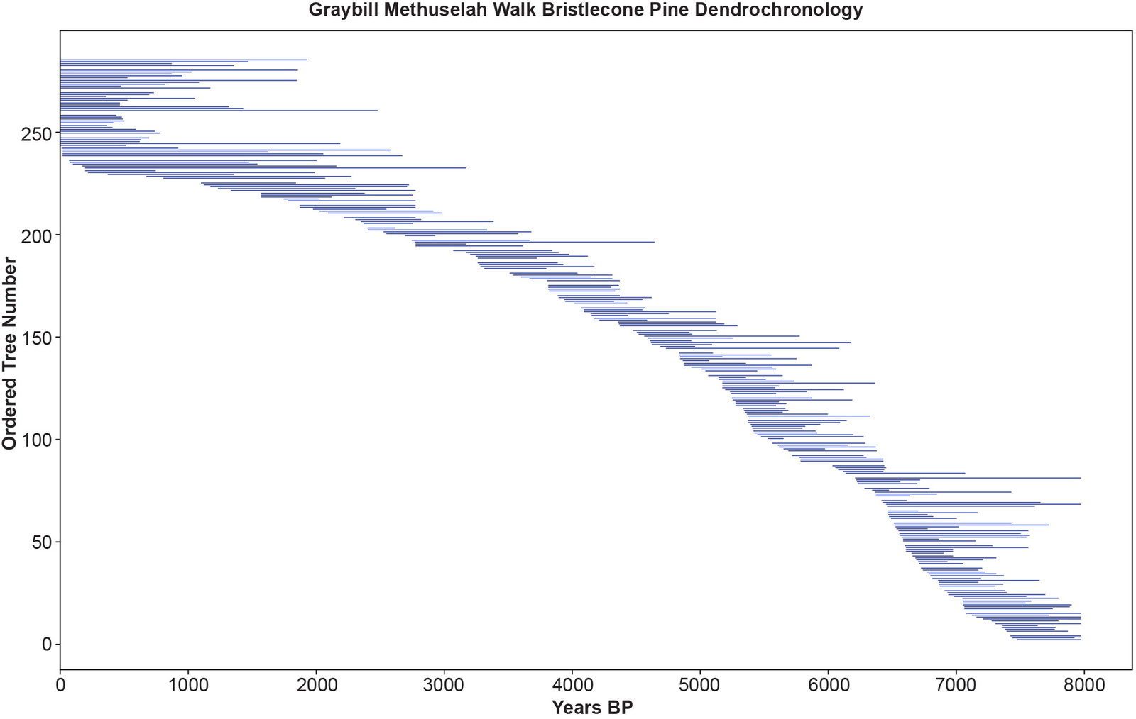
Fig. 3. The Graybill Methuselah Walk bristlecone pine dendrochronology. The y-axis is the ordered tree number of the 285 trees. The x-axis is time in years before present (BP). The length of the blue lines is proportional to each tree’s lifespan in years. There are no gaps in the dendrochronology timeline (horizontal axis). White spaces between the blue lines representing individual trees are not gaps, but these spaces allow the individual trees to be distinguished from one another. Trees bumping against the left vertical axis are living trees.

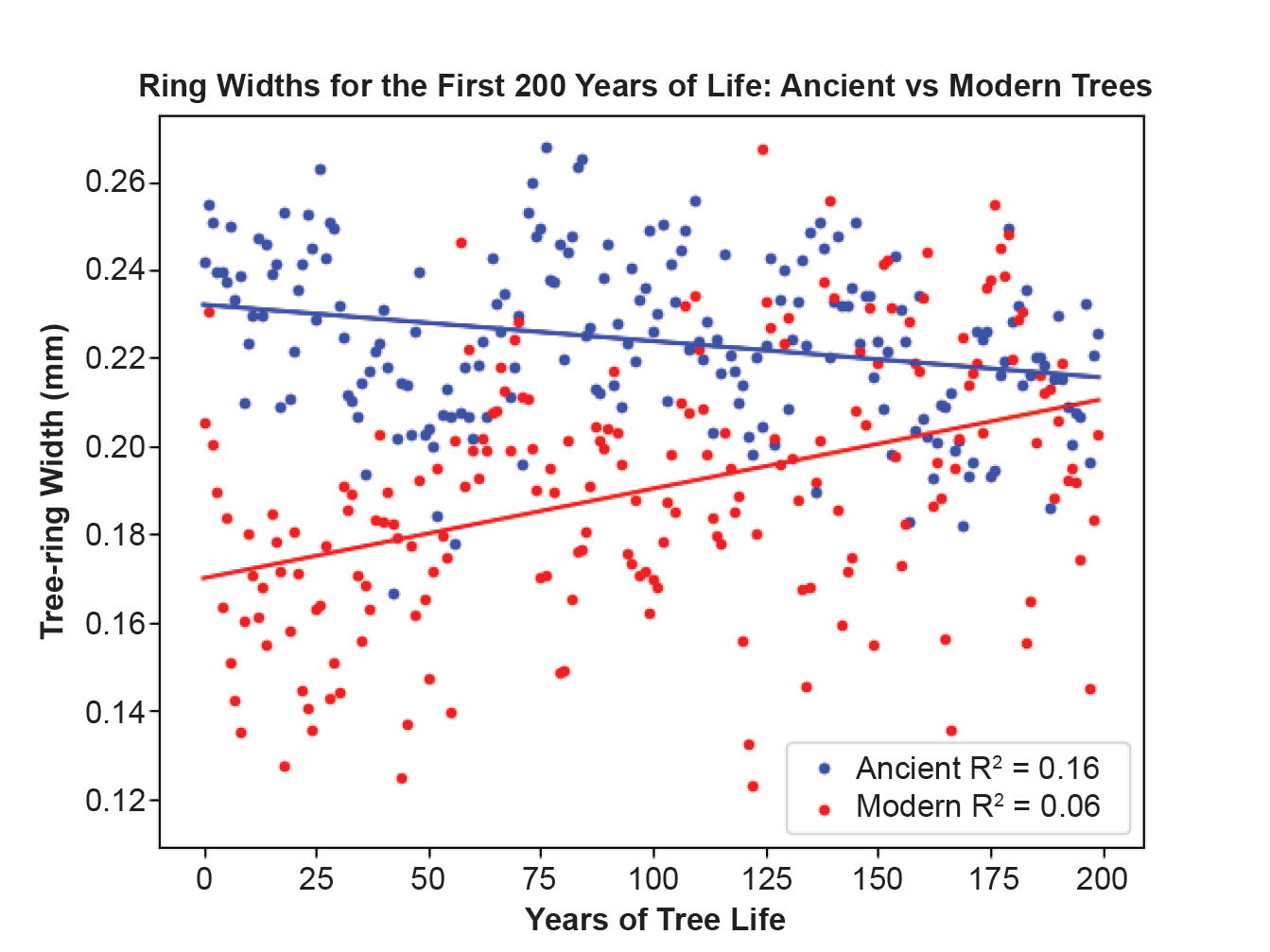
Fig. 4. Ring widths for the first 200 years of life for ancient vs modern trees in GWM data. The x-axis records years in each tree’s life span. The y-axis is the tree ring width in millimeters. The blue dots are the average ring widths for trees in the most ancient (eighth) millennium and the red dots are the average ring widths for trees in the most recent (first) millennium.

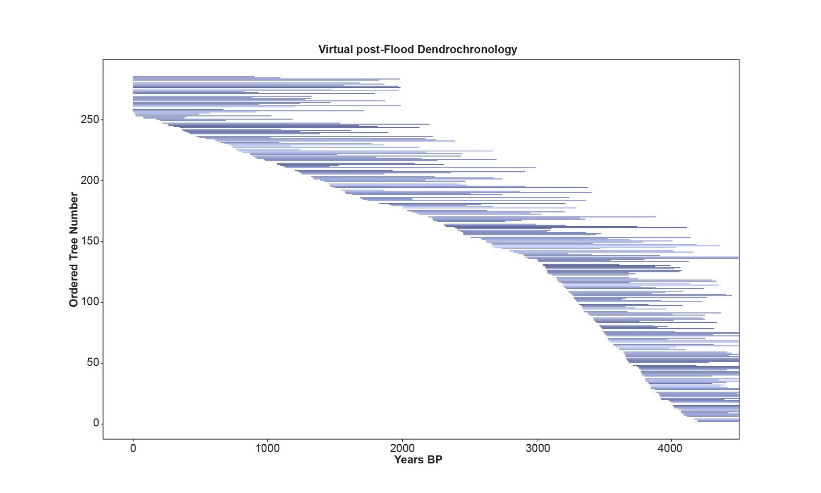
Fig. 5. The perfect virtual dendrochronology of one characteristic run of the simulation. The horizontal axis is the years before present, and the vertical axis is the 285 numbered trees of the simulation. The length of the blue lines represents the life span of the trees. There are no gaps in the dendrochronology timeline (horizontal axis). White spaces between the blue lines representing individual trees are not gaps, but these spaces allow the individual trees to be distinguished from one another. Trees aligned with 0 years BP are living trees. Trees bumping against the right vertical axis are trees that sprouted immediately after the Flood ended.

Discussion

This paper presents both a statistical analysis of the bristlecone pine dendrochronology and a simulation dendrochronology using virtual post-Flood trees. The purpose of the latter is to provide a basis for interpreting the former in the light of Scripture and a biblical timescale.

Statistical Anomalies of the Bristlecone Pine Dendrochronology

The statistical analysis was done to find any obvious weakness in the bristlecone pine dendrochronology which would render its 8,000-year length invalid. Although no such damning statistics were found, the GMW data file has some interesting anomalies which can be seen in the raw data of the Supplementary file 3. These anomalies call into question the uniformitarian assumptions on which the bristlecone pine dendrochronology is constructed.

One curious anomaly is that about 2% of all the tree rings are missing, and these are given a ring width of 0.0 in Supplementary files 7 and 8. Missing rings are inferred by the scientists who are gathering the data, and the zero-width rings are placed in the series according to strict criteria. Generally if several trees growing in a year have very thin rings, suggesting a drought, and another tree growing at the same time appears to have missed a ring, a zero-ring is inserted in that series to keep the series in phase with its contemporaries. While this may explain most of the zero-rings, it does not explain all. For example, in some years, most of the rings are missing. Could it be that when 10 trees have a zero-ring in the dataset and only one tree has a measured ring width for that year that the one tree has an extra ring rather than all the others missing a ring? Undoubtedly, this is the case for some years. But the dendrochronology does not allow for more than one ring per year, and if one tree has an extra ring in a year then all the other trees alive in that year are assigned a zero-ring as though they all had a missing ring. Interestingly, one tree (MWK691_raw) has 10% zero-rings. (See line 289 in the Supplementary file 7.

While these zero-rings raise concerns in the minds of many, Woodmorappe has studied this issue and concludes that the practice of adding zero-rings for missing rings by itself does not invalidate the bristlecone pine dendrochronology (Woodmorappe 2003a). It should be noted, however, that the oldest trees have more missing rings than the younger ones. Further, of the eight years in the chronology where more than 90% of the tree rings are missing, five of these years are in the earliest 1,500 years of the 8,000 year-long chronology. This feature certainly raises concerns among those who view this dendrochronology with skepticism. The distribution of missing rings suggests the environmental conditions affecting the growth of the bristlecone pine trees were much different from today for the older trees. Another anomaly in the data adds to this impression.

The oldest trees in the Graybill Methuselah Walk data file grew more rapidly than the youngest trees as illustrated in fig. 4. These oldest trees were growing in the first millennium after the Flood. The larger ring size in the first 200 years of life indicates faster growth under wetter conditions. This fact along with the increased zero-ring count and shorter lifespan of the most ancient trees, adds credibility to the disturbance hypothesis. Because the disturbed tree-ring series of two trees may cross-match according to the disturbance pattern when the trees were not living simultaneously, the uniformitarian assumptions of the bristlecone pine dendrochronology may not apply. There is much evidence that the oldest trees in the bristlecone pine dendrochronology grew in an environment radically different from today.

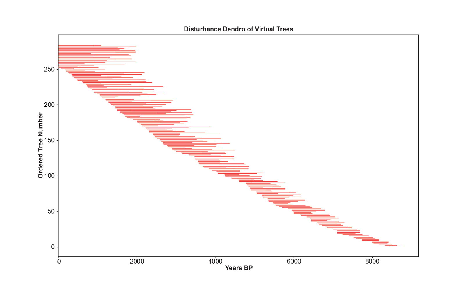
Fig. 6. The disturbance dendrochronology of one characteristic run of the simulation. The horizontal axis is the years before present, and the vertical axis is the 285 numbered trees of the simulation. The length of the red lines represents the life span of the trees. Trees aligned with 0 years BP are living trees.

That disturbance patterns may exist in the ring-width series of bristlecone pines is also suggested by the high rate of statistical cross-matching found in non-contemporaneous trees. For example, see line 28,384 in Supplementary file 11. The non-contemporaneous bristlecone pine trees cross-matched with BPTV of 5.0 or greater in 23% of cases. This greatly exceeds the 3% that are expected due to cross-matching of random series. Theoretically two trees that grew together under the same climate should demonstrate a statistically significant cross-match at only one alignment of their ring-width series (Woodmorappe 2003a). All other alignments should be insignificant, that is, with BPTV less than 5.0. However, if disturbance patterns are found in both series, then several statistically significant cross-matches might occur. Evidently 23% of the non-contemporaneous bristlecone pine trees have disturbance patterns allowing statistically valid cross-matching. This fact argues against the idea that the rings of composite series can be reliably counted back in time. To illustrate this hypothesis, the simulation presented here was devised.

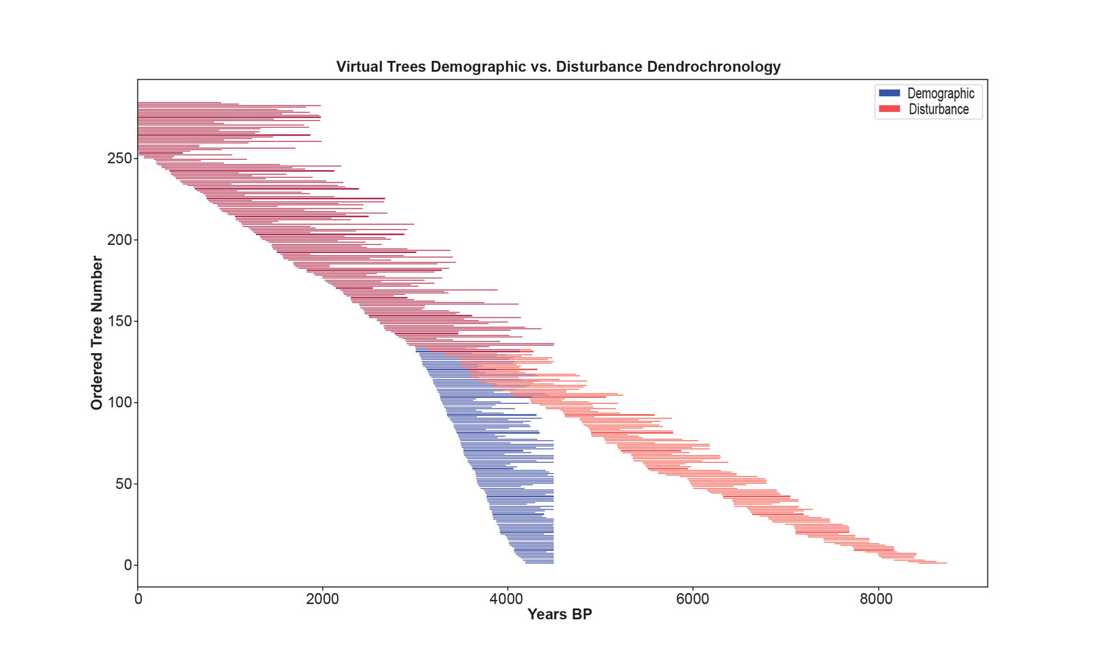
Fig. 7. The chronologies of figs. 5 and 6 displayed together. The blue lines are the virtual dendrochronology of fig. 4 which was made by cross-matching trees according to their overlaps defined by the virtual tree demographics (their sprout and death dates). The red lines are the disturbance dendrochronology of fig. 6 which was made by cross-matching the same tree pairs as in fig. 5 at all possible overlaps and orienting the trees according to the best statistics.

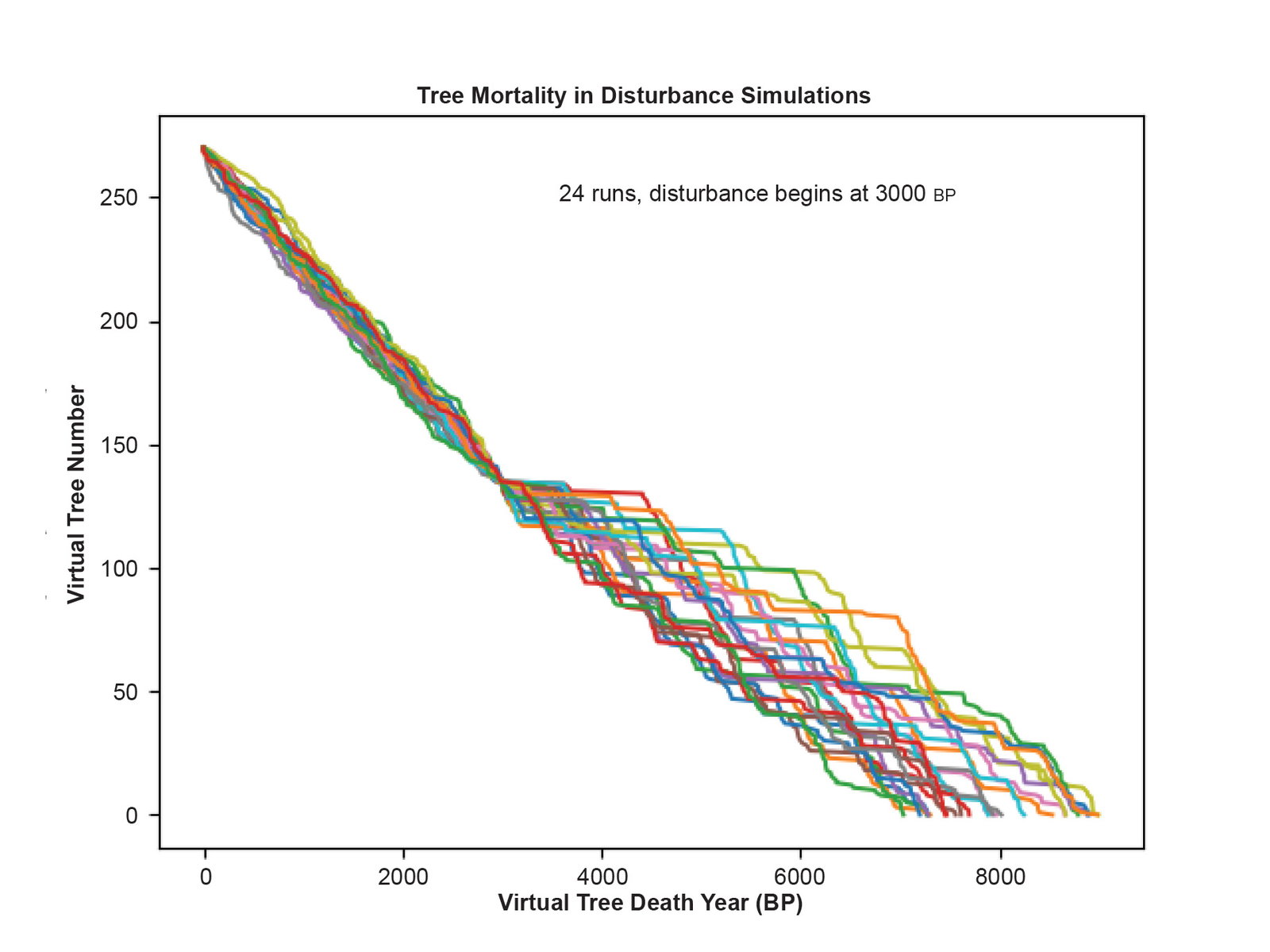
Fig. 8. Tree mortality in the disturbance simulations. Results of 24 runs of the simulation tracking just the death dates of the virtual trees when they are aligned in the dendrochronology according to cross-matching at all possible alignments. The variation in total length of each run is due to the stochastic features of the simulation.

The Simulation: How to Make a Hyper-Long Dendrochronology

The transformation of a perfect post-Flood virtual dendrochronology of 4,500-years into an 8,000-year dendrochronology is seen in table 1. Observe that the perfect virtual dendrochronology differs from the bristlecone pine dendrochronology based on these summary statistics. Because the virtual trees older than 3000 before present (BP) were designed to have a weak climate signal and a disturbance pattern, when the pairs of series are correlated based on their demographics (which aligns the series according to their contemporaneous growth years) the statistics are often very weak. By just looking at the mean PCC and mean BPTV one might think the virtual dendrochronology compares well with that of the bristlecone pines. But the magnitude of their differences is seen when one looks in table 1 at the range of the PCC and the range of the BPTV. The oldest trees in the virtual dendrochronology cross-match with statistics that fall below the threshold of significance. Examination of Supplementary file 9 reveals that many of the virtual trees older than 3000 BP correlate like a random series with BPTV less than 5.0.

The transformation of the virtual into the disturbance dendrochronology is accomplished by aligning the series based on the best BPTV values found by correlating all possible alignments. The first most recent half of both chronologies is identical because of the strong climate signal. But for the older trees in the disturbance dendrochronology, the best BPTV values occur when the series align according to the disturbance pattern which makes a statistically stronger cross-match than the weak climate signal. The disturbance pattern overwhelms the weak climate pattern.

The disturbance dendrochronology of fig. 6 gives the illusion of stretching back to several thousands of years before the date of the Flood. Of course, this can’t be true because the virtual trees from which it is constructed are all less than 4,500 years old. The horizontal axis on fig. 6 extends back to 8000 BP based on the assumption that the series have cross-matched according to the climate signal, and the combined tree rings of the dendrochronology can be counted back in time as years. However, since the disturbance pattern determines the cross-matching, the rings in the disturbance dendrochronology cannot be counted as years. As can be seen in table 1, this stretching of the virtual dendrochronology to form the disturbance dendrochronology is attended by a dramatic improvement in the summary statistics. The disturbance dendrochronology has better summary statistics than the virtual dendrochronology. It is as statistically robust as the bristlecone pine dendrochronology. For example, the lowest BPTV is 6.3 for the trees of the disturbance dendrochronology and 5.9 for the bristlecone pines dendrochronology. But this statistical validity does not prove that the disturbance dendrochronology is valid because the primary assumption, that series cross-match according to their having lived at the same time and shared the same climate features, no longer applies. The cross-matching of the older virtual trees has been dominated by the disturbance pattern which overwhelmed the weak climate signal, drawing out and lengthening the series of cross-matches without anchoring the composite series to real calendar dates.

Several other similarities and differences between the bristlecone pine dendrochronology and the simulation chronologies can be seen by comparing Supplementary file 6 to Supplementary files 9 and 10. All three show excellent PCC and BPTV values for the first recent half of the chronology. But, as noted above, for the more ancient trees the statistics in the virtual dendrochronology are very weak. Finally, the disturbance dendrochronology made entirely from post-Flood trees, mirrors the bristlecone pine dendrochronology in both length (about 8,000 years) and cross-matching statistics. Thus, the simulation presented here shows how post-Flood virtual trees, all less than 4,500 years old, can form an illusory 8,000-year dendrochronology with robust statistics based on standard cross-matching methods when disturbance patterns are present in the tree-ring series. This implies an alternative way to interpret the bristlecone pine dendrochronology.

An Alternative Interpretation of the Bristlecone Pine Dendrochronology

The 8,000-year bristlecone pine dendrochronology presents a considerable challenge to the worldview of young-earth creationists. Assuming that all subfossil trees are post-Flood, this dendrochronology should be considered wrong because it extends back beyond 4500 BP (2500 BC) the approximate date of the Flood. The question of multiple rings per year, the difficulties of measuring very thin bristlecone pine rings, and the addition of inferred missing rings have already been answered to the satisfaction of many. This paper challenges the main assumption of dendrochronology by raising this question: Does statistically valid matching of tree-ring series prove they lived at the same time and experienced the same climate features? The answer is no. Disturbance features may also cause series to cross-match with valid statistics. Because of the catastrophic global Flood, the uniformitarian assumptions of the bristlecone pine dendrochronology are inappropriate at least for dates older than 3000 BP. Therefore, the 8,000-year length assigned to this dendrochronology may be wrong. Those who believe the biblical record about the global Flood may conclude that the conditions in which trees began to grow after the Flood were radically different from today causing injury patterns in the tree rings so that they no longer cross-match according to a climate signal.

How the Flood and its Aftermath Affected Tree Growth

The description of the Flood leads one to conclude that all the trees of the pre-Flood world were buried in sediments to form the world’s coal seams. Mega-tsunamis due to catastrophic plate tectonics wiped the earth’s surface clean of all trees in much the same way that the eruption of Mount St. Helens leveled the trees around Spirit Lake with a massive wave. As the Flood waters receded, sediments buried the trees concentrated in layers where they were subsequently transformed rapidly into coal beds.

In the westernmost U.S. there were rapid tectonic adjustments at the edge of the North American plate as plate movements and subduction decelerated during the end of the Flood and through subsequent decades. This resulted in vertical tectonics as the plate edge rebounded and adjusted to form the basin and range province in which the White Mountains are located. Thus, as the White Mountains of California were uplifted by thousands of feet and shaken with violent tremors, thousands of bristlecone pine trees were sprouting out of the wet ground. This was a time of extreme vertical tectonics that resulted in relatively rapid mountain building, continental uplift, and widespread volcanism. The environmental instability would weaken the tendency of neighboring trees to grow in the same manner due to shared environmental features such as rainfall, temperature, and solar intensity. One might also expect that trees growing in shallow soil on rocky mountain sides, like the bristlecone pines of the White Mountains, could experience injury from rock falls and flash floods that would disrupt the shallow root system, causing the tree to stop growing for a time (Woodmorappe 2003b, 2009). It is this type of disturbance that serves as a model for the tree-ring disturbance patterns used in the simulation presented in this paper. Fig. 9 illustrates the supposed disturbance of trees growing on the unstable slopes of the White Mountains.

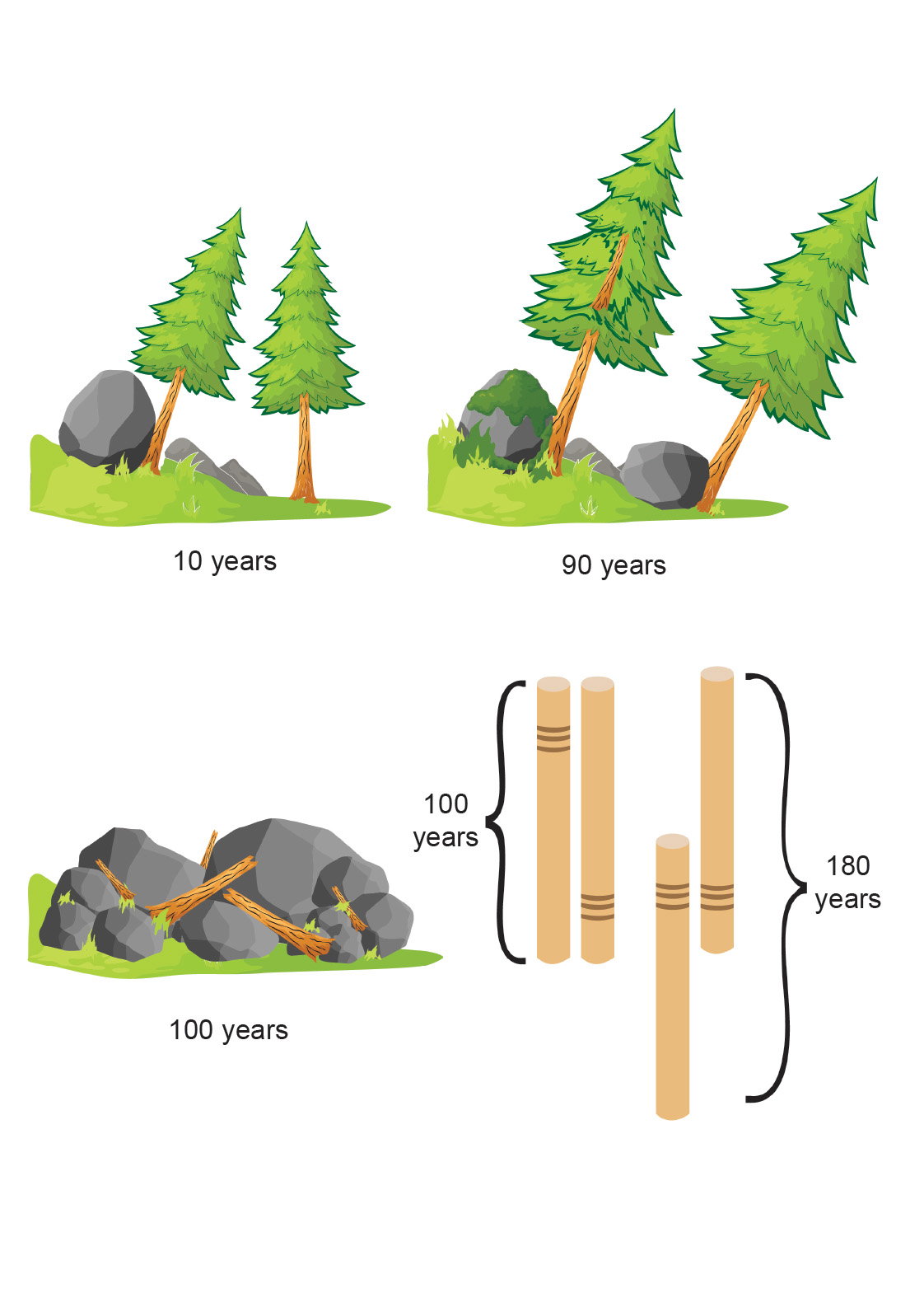
Fig. 9. An illustration of tree disturbance caused by rockfalls causing two trees that grew contemporaneously for 100 years to cross-match as though their lives spanned 180 years.

In fig. 9, one potential cause of a tree-ring disturbance pattern is illustrated. A large boulder dislodged by a tremor on the steep White Mountains slope crashes into the trunk of a young tree ten years after it sprouted dislodging its shallow root system that is growing in the thin, rocky soil. This causes the tree to stop growing for several years producing thin or absent rings. When the tree recovers from the injury, it returns to normal growth. Eighty years later the same disturbance afflicts a neighboring tree causing it to stop growing which produces the same disturbance pattern. Both trees then die in a landslide at age 100 years. When the series of these contemporaneous dead trees are cross-matched, if they align properly for the 100 years they lived together, their composite series will span only 100 years. But they align according to the disturbance pattern, giving a false impression that their combined series spanned 180 years. If this sort of scenario occurred in just a few of the older bristlecone pine trees causing their series to cross-match in a time-transgressive manner, the chronology would be extended far beyond the dates the trees lived.

Besides slope instability and rock falls, the growth of trees may have been disturbed by other unique events in the early post-Flood world. For example, atmospheric carbon dioxide may have been highly variable immediately after the Flood. Under the fresh Flood sediments plants and animals were rotting potentially releasing carbon dioxide. Since carbon dioxide acts like a fertilizer to accelerate tree growth (de Boer et al. 2019; Laffitte et al. 2023), the release of carbon dioxide could cause some trees to grow rapidly and add rings while neighboring trees may not have been affected (Woodmorappe 2003a). Many speculations of this nature can be imagined since we know little about the post-Flood environment of the White Mountains. But this emphasizes the main point: the uniformitarian assumptions of the bristlecone pine dendrochronology are not justified given the likely post-Flood environmental instability.

Another possible disturbance to the ancient trees could be insect infestations that affect one tree but not the neighboring trees. It has long been known that cyclical insect infestations can produce anomalous tree-ring series. Examples include infestations with the larch budworm (Fan and Bräuning 2017), the eastern spruce budworm, the forest tent caterpillar, and the common cockchafer ( Melolontha melolontha) among others (Aryal et al. 2023; Dechaine et a. 2023; Kolář, Rybníček, and Tegel 2013). When a tree is defoliated by insects, it stops growing producing a narrow or absent ring. Dendrochronologists are aware that infestations may be cyclical as the insects return regularly, and they are watching for such repetitive disruption patterns in the tree rings (Friedrich et al. 2004). But what if the infestations are random and localized afflicting one tree but not its neighbor? This could cause disturbance patterns in the trees at different times so that they cross-match in a “time transgressive” manner falsely lengthening the chronology. The disturbed tree-ring series caused by cyclical infestations can be identified and discarded from use in a dendrochronology. But in the unstable post-Flood environment, insect infestations may have been random and their telltale disturbance patterns hidden in the tree-ring series.

All these potential differences from today’s environment in the White Mountains serve to counter the primary assumption of the bristlecone pine dendrochronology. Furthermore, anomalies in the bristlecone pine data support the idea that the environment in which the oldest subfossil trees grew was unstable and unlike today’s environment.

What About Multiple Rings Per Year?

It is possible that the post-Flood environment could have caused bristlecone pines to form multiple rings per year. This fact alone would negate the chronology’s excessive length. Two rings per year across that entire chronology would cut it in half and move all the bristlecone subfossil trees to the post-Flood era. But this solution is unacceptable to those who have devoted their careers to the study of the bristlecone pines of the White Mountains of California. Nearly all researchers insist that bristlecone pines in the White Mountains never form more than one annual ring. Although it has been demonstrated that bristlecone pine seedlings grown experimentally under various conditions can be induced to form multiple rings per year (Lammerts 1983), the required conditions are dissimilar to those that prevail in the White Mountains today. This leads uniformitarian scientists to dismiss this multiple-ring objection. But the claim that no multiple rings formed in the past because no multiple rings are forming today, is simply a bold uniformitarian assertion made by those who ignore the Genesis record of the Flood.

Conclusion

The hyper-long bristlecone pine dendrochronology provides yet another example of how scientists apply uniformitarian assumptions in their attempts to understand earth’s history without reference to the biblical record. They assume that tree-ring patterns of long-dead trees cross-match for the same reason that modern tree ring patterns cross-match: the trees must have grown at the same time under similar environmental conditions. This assumption is questionable because trees growing soon after the Flood faced radically different conditions than those prevailing today. Disturbance patterns produced in the tree rings may cause them to cross-match with strong statistics, but this does not allow the combined series of rings to be counted as a yearly record. The simulation using post-Flood virtual trees shows how disturbance patterns can make a statistically robust 8,000-year dendrochronology from trees less than 4,500 years old. Statistical analysis of the simulated disturbance dendrochronology mirrors the bristlecone pine dendrochronology. Both have very strong cross-match statistics. While this simulation does not overturn the validity of the bristlecone pine dendrochronology, it does provide an alternative explanation for its apparent 8,000-year length. Thus, Christians need not be tempted to doubt the historical record of Genesis simply because scientists who ignore the Bible can make dead bristlecone pine trees form a dendrochronology stretching back before the Flood.

One does not need the wisdom of Solomon to discern that those who reject the biblical record of the Flood will fail to correctly understand earth’s history. Since the fear of the Lord is the beginning of wisdom (Proverbs 9:10), the bristlecone pine dendrochronology must be interpreted in the light of Scripture.

References

Aryal, Sugam, Jussi Grießinger, Mohsen Arsalani, Wolfgang Jens-Henrik Meier, Pei-Li Fu, Ze-Xin Fan, and Achim Bräuning. 2023. “Insect Infestations have an Impact on the Quality of Climate Reconstructions Using Larix Ring-Width Chronologies from the Tibetan Plateau.” Ecological Indicators 148 (April): 1–12.

Baillie, M. G. L., and J. R. Pilcher. 1973. “A Simple Crossdating Program for Tree-Ring Research.” Tree-Ring Bulletin 33: 7–14.

de Boer, Hugo J., Iain Robertson, Rory Clisby, Neil J. Loader, Mary Gagen, Giles H. F. Young, Friederike Wagner-Cremer, Charles R. Hipkin, and Danny McCarroll. 2019. “Tree-Ring Isotopes Suggest Atmospheric Drying Limits Temperature-Growth Responses of Treeline Bristlecone Pine.” Tree Physiology 39, no. 6 (June): 983–999

Becker, Bernd. 1993. “An 11,000-year German Oak and Pine Dendrochronology for Radiocarbon Calibration.” Radiocarbon 35, no. 1: 201–213.

Bernabei, Mauro, and Pietro Franceschi. 2025. “Reconsidering the Use of t-Statistics in Dendroprovenancing.” Dendrochronologia 91 (June): Article no. 126332.

Brown, R. H. 1968. “Radiocarbon Dating.” Creation Research Society Quarterly 5, no. 2: 65–68, 87.

Dechaine, Andrew C., Douglas G. Pfeiffer, Thomas P. Kuhar, Scott M. Salom, Tracey C. Leskey, Kelly C. McIntyre, Brian Walsh, and James H. Speer. 2023. “Dendrochronology Reveals Different Effects Among Host Tree Species from Feeding by Lycorma delicatula (White).” Frontiers in Insect Science 3 (1 September): Article number 1137082.

Douglass, Andrew Ellicott. 1929. “The Secret of the Southwest Solved by Talkative Tree Rings.” National Geographic 56, no. 6 (July–December): 737–770.

Fan, Ze-Xin, and Achim Bräuning. 2017. “Tree-Ring Evidence for the Historical Cyclic Defoliator Outbreaks on Larix potaninii in the Central Hengduan Mountains, SW China.” Ecological Indicators 74 (March): 160–171.

Ferguson, C. W. 1969. “A 7104-Year Annual Tree-Ring Chronology for Bristlecone Pine, Pinus aristata, from the White Mountains, California.” Tree Ring Bulletin 29, nos. 3–4 (August): 3–29.

Ferguson, C. W. 1979. “Dendrochronology of Bristlecone Pine, Pinus longaeva.” Environmental International 2, nos. 4–6: 209–214.

Friedrich, Michael, Sabine Remmele, Bernd Kromer, Jutta Hofmann, Marco Spurk, Klaus Felix Kaiser, Christian Orcel, and Manfred Küppers. 2004. “The 12,460-year Hohenheim Oak and Pine Tree-Ring Chronology from Central Europe—A Unique Annual Record for Radiocarbon Calibration and Paleoenvironment Reconstructions.” Radiocarbon 46, no. 3 (18 July): 1111–1122.

Hebert, Jake, Andrew A. Snelling, and Timothy Clarey. 2016. “Do Varves, Tree-Rings, and Radiocarbon Measurements Prove an Old Earth? Refuting a Popular Argument by Old-Earth Geologists Gregg Davidson and Ken Wolgemuth.” Answers Research Journal 9 (7 December): 339–361. https://answersresearchjournal.org/varves-trees-radiocarbon-old-earth/.

Keenan, Douglas J. 2006. “Anatolian tree-ring studies are untrustworthy.” Academia.edu. https://www.academia.edu/7991497/Anatolian_tree_ring_studies_are_untrustworthy

Kolář, T., M. Rybníček, and W. Tegel. 2013. “Dendrochronological Evidence of Cockchafer ( Melolontha sp.) Outbreaks in Subfossil Tree-Trunks from Tovačov (CZ Moravia).” Dendrochronologia 31, no. 1: 29–33.

Laffitte, Benjamin, Barnabas C. Seyler, Pengbo Li, Zhengang Ha, and Ya Tang. 2023. “Using Tree-Rings to Detect a CO ₂ Fertilization Effect: A Global Review.” Trees: Structure and Function 37 (5 August): 1299–1314.

Lammerts, Walter E. 1976. “Evidence of Cyclic Variation in Tree Rings.” Creation Research Society Quarterly 13:172.

Lammerts, Walter 1983. “Are the Bristle-Cone Pine Trees Really So Old?” Creation Research Society Quarterly 20, no. 2 (September): 108–115.

Larson, Lars-Ake. 2021. “Cybis Dendrochronology.” Cybis Elektronik & Data AB. https://www.cybis.se/forfun/dendro/index.htm.

Larsson, Petra Ossowski, and Lars-Ake Larsson. 2018. “Validation of the Supra-Long Pine Tree-Ring Chronologies from Northern Scandinavia.” Scand. Pine reference building, draft, 2018-01-23: 1–11. https://www.researchgate.net/publication/322662787_Validation_of_the_supra-long_pine_tree-ring_chronologies_from_northern_Scandinavia.

McPartland, M. Y., S. St. George, Gregory T. Pederson, and Kevin J. Anchukaitis. 2020. “Does Signal-Free Detrending Increase Chronology Coherence in Large Tree-Ring Networks?” Dendrochronologia 63 (October): Article number 125755.

Miller, Hugh G., and Jean M. Cooper. 1976. “Tree Growth and Climatic Cycles in the Rain Shadow of the Grampian Mountains.” Nature 260, no. 5553 (22 April): 697–698.

Pearson, Charlotte L., Steven W. Leavitt, Bernd Kromer, Sami K. Solanki, and Ilya Usoskin. 2022. “Dendrochronology and Radiocarbon Dating.” Radiocarbon 64, no. 3 (3 December): 569–588.

Pilcher, J. R., M. G. L. Baillie, B. Schmidt, and B. Becker. 1984. “A 7,272-Year Tree-Ring Chronology for Western Europe.” Nature 312, no. 5990 (8 November): 150–152.

Reimer, Paula J., William E. N. Austin, Edouard Bard, Alex Bayliss, Paul G. Blackwell, Christopher Bronk Ramsey, Martin Butzin, et al. 2020. “The IntCal20 Northern Hemisphere Radiocarbon Age Calibration Curve (0–55 cal kBP).” Radiocarbon 62, no. 4 (August): 725–757.

Ricker, Martin, Genaro Gutiérrez-García, David Juárez-Guerrero, and Margaret E. K. Evans. 2020. “Statistical Age Determination of Tree Rings.” PLoS One 15 no. 9 (September 22): e0239052.

Sanders, Roger W. 2018. “Creationist Commentary on and Analysis of Tree-Ring Data: A Review.” In Proceedings of the Eighth International Conference on Creationism. Edited by John H. Whitmore, 516–524. Pittsburgh, Pennsylvania: Creation Science Fellowship.

Schulman, Edmund. 1954. “Longevity Under Adversity in Conifers.” Science 119, no. 3091 (26 March): 396–399.

Snelling, Andrew A. 2017. “Layers of Assumptions: Are Tree Rings and Other ‘Annual’ Dating Methods Reliable?” Answers 12, no. 1 (January 1): 54–63.

Sorensen, Herbert C. 1976. “Bristlecone Pines and Tree-Ring Dating: A Critique.” Creation Research Society Quarterly 13, no. 1 (June): 5–6.

Woodmorappe, John. 2003a. “Collapsing the Long Bristlecone Pine Tree Ring Chronologies.” In Proceedings of the Fifth International Conference on Creationism. Edited by Robert L. Ivey, Jr., 491–504. Pittsburgh, Pennsylvania: Creation Science Fellowship.

Woodmorappe, John. 2003b. “Field Studies in the Ancient Bristlecone Pine Forest.” TJ 17, no. 3 (December): 119–127.

Woodmorappe, John. 2009. “Biblical Chronology and the 8,000-Year-Long Bristlecone Pine Tree-Ring Chronology.” Answers in Depth 4: 4–5. https://assets.answersingenesis.org/doc/articles/aid/v4/biblical-chronology-bristlecone-pine.pdf.

Woodmorappe, John. 2018. “Tree Ring Disturbance-Clustering for the Collapse of Long Tree-Ring Chronologies.” In Proceedings of the Eighth International Conference on Creationism. Edited by John H. Whitmore, 652–672. Pittsburgh, Pennsylvania: Creation Science Fellowship.