The views expressed in this paper are those of the writer(s) and are not necessarily those of the ARJ Editor or Answers in Genesis.
Abstract
Modern biology has come to realize that all life is built upon information stored within DNA. Until now, discussions of genetic information have relied almost exclusively on models of information that do not use variables. The result is that a scientific understanding of life is hindered, because investigations are based on inaccurate models of biological information.
By contrast, the Bible’s description of created kinds implies an information model which uses variables. The findings in this paper show that a model which uses variables forms a stronger basis for true scientific understanding of biology and, by implication, the Bible provides a superior foundation for scientific investigation. In addition, the paper is able to propose a definition of biblical kinds based upon an information model which uses variables.
Keywords: DNA, variables, genetics, programming languages, evolution, baraminology
Introduction
The fundamental issue in the debate over evolution is whether or not the variation we see within populations can accumulate over time to result in new kinds of organisms. Evolutionists say yes while biblical creationists say no. The evolutionary world view can be seen when Travis and Reznick state, “Darwin argued that macroevolution is just microevolution writ large, or that the process we see and study as the cause of microevolution will, given sufficient time, also cause everything that we attribute to macroevolution.” (Travis and Reznick 2009, p. 126).
However, Darwin’s argument clearly ignores the biblical revelation of created kinds (Genesis 1:11–27) in favor of human wisdom. As the Bible states, “They exchanged the truth about God for a lie, and worshiped and served created things rather than the Creator—who is forever praised. Amen.” (Romans 1:25)
Independent of the specific mechanisms evolutionists cite, the tie between microevolution and macroevolution is necessarily dependent upon the fundamental idea that “heritable differences . . . accumulate . . . eventually giving rise to the larger differences between species and higher taxa” (Silvertown 2009, p. 29). This notion of accumulated change leads to the conclusion that “All organisms are related by common descent from a single form of life” (Ayala 2009, p. 133). This common descent, sometimes referred to as universal common descent, is often pictured as a tree of life (Ayala 2009). Different authors may give the tree slightly different shapes, but it’s still a tree (Futuyma 1986; Ruse and Travis 2009). In contrast, the biblical kinds are sometimes pictured as a lawn or orchard as opposed to a tree (Patterson 2006).
For the purpose of this paper I define an evolutionist as anyone who holds to the idea of common descent. Note that this definition is not limited to naturalists, but includes anyone who holds to common descent. This can include Intelligent Design proponents and creationists. Though evolutionists may debate the mechanisms, they all hold to the man-made idea that one kind of organism can change into another. Common descent, by definition, rejects the idea that life consists of bounded sets which cannot be bridged by inheritance.
However, descent from a common ancestor has never been observed. It is simply an interpretation of externally observed differences, based on an evolutionary world view. The biblical world view interprets the exact same externally observed differences as variation within unchanging kinds and claims that evolution does not happen.
The Bible tells us in 2 Corinthians 10:5 that we should “take captive every thought.” Proverbs 14:12 says, “There is a way that seems right to a man, but in the end it leads to death.” I do not mean to imply that Proverbs 14:12 is expressly about evolution, but it is interesting that evolution is all about death and it definitely seems right to men. Clearly the fundamental principle in both these verses is that man’s thinking alone cannot be trusted and must be subjected to God’s revelation in the Bible.
When we start with the Bible as our basis for understanding biology, we find that God created the organisms of the world “after their kind” (Genesis 1). That language continues in the account of the flood, when God says, “And of every living thing of all flesh, you shall bring two of every kind into the ark, to keep them alive with you; they shall be male and female. Of the birds after their kind, and of the animals after their kind, of every creeping thing of the ground after its kind, two of every kind will come to you to keep them alive.” (Genesis 6:19–20)
If evolution is true, then kinds are only transitory observational conveniences, because they are simply snapshots of organisms transitioning through history. However, the language of Genesis 1 and 6 implies that kinds are an enduring organizational structure through which God views the life He created. Contrary to evolutionary thinking, which sees heritable differences as changes in the essence of organisms, the Bible paints a picture of life composed of bounded groups or sets called kinds, where heritable differences are simply variations within those kinds. One common misconception is to equate species with biblical kinds (Milner 1990), but this is neither biblically nor scientifically accurate. The Bible does not describe how kinds are defined, but clearly states that they exist and never implies evolution in the text.
Because every word of God is true (Numbers 23:19; 2 Timothy 3:16–17) we expect DNA to be best described by an information model which allows variation within bounded kinds. Although existing work has already successfully shown that meaningful messages do not arise from random processes (Bradley and Thaxton 1994; Gitt 2007; Riddle 2009; Spetner 1997) and even shown that the existence of meaningful messages implies an intelligent author (Gitt 2007), they do not examine the question of how different models of information explain variation and how that variation can be bounded.
This paper examines how variation occurs within different information models and considers their implications with respect to both structures within the cell and observed external differences in organisms. It shows that without variables, variation is equivalent to evolution, but basic scientific observations cannot be explained. On the other hand if a system uses variables, variation is bounded and biological observations can be easily explained. In such systems variation does not accumulate to result in evolution. Thus, variation is not simply evolution limited by the improbability of creating information through random means. In models that use variables, variation is a fundamentally different informational property than evolution and leads to a proposed definition of biblical kinds.
Modification: The Evolutionary View of Variation
The evolutionary world view sees variation as modification. The child’s DNA is just a modification of the parent’s DNA. This is why, when seeing nothing more than variation in the peppered moth population, Bernard Kettlewell, “called industrial melanism in peppered moths ‘the most striking evolutionary change ever actually witnessed in any organism.’” (Wells 2002, p. 143) When it was discovered that DNA contained “the instructions for life” (Palladino 2006) evolutionists did not question their assumption of common descent, but simply assumed that instructions could evolve in a way to match their a priori assumption. The assumption that DNA is simply a sequence of accumulated modifications is seen in statements such as those by Michael Behe,
Evolution from a common ancestor, via changes in DNA, is very well supported . . . scientists who sequence human DNA . . . are actually observing the results of a struggle that’s gone on for millennia (Behe 2007, p. 12).
In Darwin’s Black Box Behe argues eloquently for design in the origin of biological machines, and notes that this understanding came as science moved from general postulations to an accurate elucidation of the actual structures and operations in biological molecules (Behe 1996). Unfortunately, he does not apply the same rigor in his thinking of information when he speaks of sequencing DNA. Just as it was important to look deeply into the actual structure of molecular machines to gain real understanding, we must go far beyond simple sequence comparisons of DNA if we hope to have a full understanding of how DNA functions.
Random sequence model
Virtually every discussion of DNA recognizes it as a sequence of code symbols, so let’s begin by asking the question, “Is DNA just a random sequence of symbols, where nearly all sequences will be reproduced and can compete in natural selection?”
Whether they’re aware of it or not, this is the model used by Richard Dawkins’ biomorph program (Dawkins 1996) and the Avida program (Lenski et al. 2003), because both systems are designed to allow random modification. In nearly all cases the modifications do not affect the ability of the organism to survive and reproduce. In this model variation is achieved by mutating symbols in the sequence. This model aligns with evolution, because the entire sequence is either open to change or is common to all sequences so it is appropriate to say that the essence of the sequence is evolving.
The problem, from a biological perspective, is that explaining variation as modifications to a random sequence cannot explain simultaneous variation and stasis. We can see this by looking at random mutations to an arbitrary sequence as shown below.
CTTGACAGGC
CTCGATAGTC
ATCCATTCTA
Notice that divergence will happen as quickly as variation, because they are explained by the same mechanism. Evolutionists might claim that stasis can be explained by natural selection favoring a specific form for a time. This may be true, but the point being discussed here is that simultaneous variation and stasis cannot be explained by the information model itself, because if variation is happening, so is divergence. If divergence is not happening, then neither is variation.
The importance of stasis is noted by Gould when he states that the “. . . cardinal and dominant fact of the fossil record” is that “the great majority of species appear with geological abruptness in the fossil record and then persist in stasis until their extinction.” (Gould 2002, p. 749)
Strictly speaking Gould is referring to stasis as viewed from phenotype. It is beyond the scope of this paper to address the relationship between phenotype and genetic sequence, but I do contend that stasis and variation can be measured at the genetic level. Therefore, in this paper when I speak of variation and stasis, I am meaning as viewed at the genetic level.
The inability to model simultaneous variation and stasis makes the random sequence model a poor model for DNA. But, perhaps an even more important problem with modeling variation as modifications to a random sequence of symbols is that research has shown that DNA is not random (Bodmer and McKie 1995; Bradley and Thaxton 1994; Whitfield 1993). This has led some researchers to model DNA as a sentence.
Sentence model
Some discussions of DNA speak of it as a language composed of words (Bodmer and McKie 1995; Bradley and Thaxton 1994; Whitfield 1993). Others compare it directly to sentences (Dawkins 1996). So, “Is DNA like a sentence or a collection of sentences?”
Like the random sequence model, the sentence model aligns with evolution. Again, variation is achieved by mutating symbols in the sentence. The entire sentence is open to change, so it is appropriate to say that the essence of the sentence is evolving.
Modeling DNA as a set of sentences is superior to the random sequence model, because it does recognize that DNA is similar to written languages in its non-random nature. Bradley and Thaxton refer to this as specified complexity (Bradley and Thaxton 1994). However, the sentence model has a number of problems. The most obvious problem is that natural language sentences cannot be fully apprehended by computers and used for their instruction (I will refer to this as machine readable). Behe shows that “life is based on machines—machines made of molecules” (Behe 1996, p. 4). It is these machines which operate on DNA (Behe 1996; Lester and Bohlin 1989) so DNA is best modeled by a language which is machine readable.
We do know of machine readable languages (Aho, Sethi, and Ullman 1986), so this point can be overcome, but it does mean that arguments based on sentences may be false, because they are based on weak analogy (Bluedorn and Bluedorn 2003). A good example is Dawkins’ illustration of cumulative selection, implying that sentences with spelling mistakes are examples of valid steps toward new information (Dawkins 1996). This is not true, because a machine cannot recognize what was intended by the author. Very often a single spelling mistake is fatal for machine languages (Perry 1993).
This brings us to perhaps the biggest challenge of the sentence model. Sentences cannot, in general, be randomly mutated. In the sentence model, as in the random sequence model, variation must occur by mutating an existing sequence. However, the sentence model has the added constraint that specified complexity must be maintained. The problem is, as we noted in the introduction, that research has clearly shown that meaningful messages do not arise from random processes (Bradley and Thaxton 1994; Gitt 2007; Spetner 1997). In fact the evidence is so strong that it is stated as the First Law of Information:
First Law of Information (LI1)
Information cannot originate in statistical processes. (Chance plus time cannot create information no matter how many chances or how much time is available.)
There is no known law of nature, no known process, and no known sequence of events which can cause information to originate by itself in matter (Riddle 2009, p. 202).
The reader needs to understand that the issue is not just the difficulty of changing one word in a sentence to another, for example from “bat” to “cat,” and have the sentence continue to make sense with no spelling mistakes. The true problem that the first law is getting at is the meaning and intention of a brand new sequence of symbols (Gitt 2007). If I introduce a new sequence of symbols, “ahkllj,” what does that mean? The words “bat” and “cat” and every other word in the sentence only have meaning, because intelligent beings defined their meaning (Gitt 2007).
What we find is that sentences are a poor model of DNA, because sentences explain variation as modification, but the First Law of Information tells us that natural processes cannot create modifications with specified complexity. Thus, the First Law of Information must be violated in order to explain variation, if DNA is modeled by the sentence model of information. The problem is even further exacerbated by the fact that a sentence model does nothing to answer the problem of simultaneous variation and stasis we found with random sequences. This brings us to a critical decision point with respect to the human idea of common descent. If we cannot create information through natural forces then common descent cannot be explained either.
At this point those who demand a naturalistic explanation for everything not created by man are stuck. Modeling variation as modifications to a random sequence or a set of sentences aligns so well with the evolutionary world view that evolutionary scientists have used these models unquestioningly to represent DNA. They have not even stopped to ask whether or not sequences and sentences are the most accurate models of information in DNA. As a result the evolutionary world view has actually hindered scientific understanding. Like their continuing quest for transitional forms in the fossil record, committed naturalists will continue to search for ways to create information through natural forces and ignore the clear signs of science rather than reconsider their assumption of common descent.
On the other hand, for anyone willing to follow the truth when it points to the God of the Bible, there is a more elegant solution. It does require abandoning the prevailing god of common descent, but it leads to a model that explains rapid variation as well as stasis without a violation of the First Law of Information. More importantly it points us to the Intelligent Designer who has written information not only in biology, but also in His Word, telling us of His creation of organisms “according to their kinds” (Genesis 1).
Variables: A Biblical View of Variation
In Proverbs 4:7b the Bible says, “Though it cost all you have, get understanding.” To gain understanding in biology we must base our thinking on what the Bible has to say. Some theists and Intelligent Design proponents may try to marry human thinking with divine revelation by proposing that God created through evolution, whether from one ancestor or many. However, as a friend said to me when I was in college, “That’s not what the Bible says.” Common descent is the illusion that must be abandoned, not biblical kinds.
As we saw in the introduction, biblical kinds imply bounded variation. We have also seen that modifications to sequences or sentences cannot explain variation without violating stasis and the First Law of Information. So the obvious question is, “How can we explain variation from a biblical world view?” The answer is variables. Variables are used by equations and computer programs to generate many different outputs without altering the equation or program itself. A computer program is a type of complex mathematical equation. It contains variables, but it also is machine readable. As a result computer programs align well with biblical revelation and are the model I propose for DNA.
The computer program model
Sometimes DNA is likened to a computer program or a set of instructions (Palladino 2006). These references hint at computer programs as a model for DNA. However, the literature has yet to look at the properties that are unique to computer programs, as compared to random sequences or sentences, and what those properties might imply.
For this paper I define the computer program model as the representation of DNA as a functional computer program where both data and instructions are combined in a single stream. A stream is simply a series of symbols of undetermined length. In an informal way you can think of the data as the variables, but in a technical sense the variable is part of the instructional code and the data is the value that will be assigned to the variable (Aho, Sethi, and Ullman 1986; Mansfield 2009).
In this definition I am specifically looking at the highest level of abstraction of a computer program. Computer programs can actually be treated as data by other programs such as compilers, operating systems, and text editors, but these are levels of abstraction. Using abstraction, computer programs can also dynamically load, move and control portions of instruction code, called subroutines or functions, during execution to perform their job. It is even possible for computer programs to generate sections of programming code on the fly, turn them on and off and call them in different orders, but it is always a computational result of information at a higher level created by an intelligent being or beings. No matter how many layers of abstraction you have in a computer system, there is always a top level instruction set that controls everything below it and must be the result of a creative mind.
As Gitt states,
Computer software functions according to this principle, since all creative ideas like algorithms (methods of solution) and data structures had to be devised beforehand by the programmer and then implemented in the form of a written program. The various relevant parameters can be entered into a machine (computer) which does nothing more than reproduce the available information in the required form. Even the results obtained by means of AI programs (artificial intelligence; see appendix A2.3) are in the last instance nothing more than reproduced information. They may be quite complex and may appear to be ‘intelligent,’ but they cannot create information [sic] (2007, p. 112).

Fig. 1. A sentence can be thought of as a sequence of symbols with the additional constraint that it has specified complexity. Similarly, a computer program can be thought of as a sentence with the additional constraints that it is machine readable and has variables. The concept of variables is critical to the evolutionary question, because it explains why incredible variation can exist within a kind without evolution occurring.
In the computer program model this principle implies that the top level of instructions is fixed and invariant (immutable) in accordance with the First Law of Information. This does not mean that the instructions cannot move within the stream or that mutations cannot cause them to degrade or fail, but that they cannot be modified by statistical processes to create a new computer program (new information) and they are not open to data substitution (which is what separates the top level instruction portion from the data portion of a computer program).
The key point to remember, in this discussion, is that a computer program does have variables, but random symbol sequences and sentences do not. As a result there is an informational structure in the computer program model, not found in either a random symbol sequence or a set of sentences, which allows variation without altering the fundamental essence defining the kind. At the sequence level this means that there is a construct in the model allowing machines to separate the entire sequence into two fundamentally distinct portions (even if they are subdivided and interleaved within the physical stream). One portion remains constant over all instances (members of the kind) and the other is open to variation (through data substitution). Fig. 1 shows the key distinction between a random symbol sequence, a sentence, and a computer program.
Mansfield expresses the separation of data and instructions when he states
Computers use two primary types of information: data and programming. Data is raw information . . . . Programming is a series of instructions describing how to manipulate data (Mansfield 2009).
As we shall see, the separation of data from instructions as part of the language is what allows the computer program to support simultaneous variation and stasis while honoring the First Law of Information.
Contrary to the random sequence model and the sentence model, which depend upon modifications to explain variation, the computer program model explains variation by data substitution. To get variation we substitute one piece of data for another of the same type. Different variations are created by combining different pieces of existing data, not by creating new segments of information. We can look at the computer program model is a type of template. The top level instruction portion of the stream is fixed and does not vary. This is the portion that holds the functional information common to all members of the kind. The data, however, can be substituted, or replaced, by any data of an equivalent type. This is because the computer program model uses variables while the random sequence model and the sentence model do not.
To illustrate this simply, consider the equation:
a + b = c
Each variable, “a,” “b,” and “c” is like a blank that can be filled in with data. If we substitute data values for each variable we get a set of equations.
1 + 2 = 3
4 + 6 = 10
38 + 124 = 162
If you view an equation as just a sequence of symbols or as just a mathematical sentence you may say that the equation is evolving. However, if you recognize that there is a difference between the functionality (operators) and the data (operands) you will see that even though variation is occurring, the equation is not evolving. The equation is always functionally exactly the same. The essence of the equation remains fixed no matter what data is substituted into the variables. In fact an equation cannot evolve by altering the data.
Like an equation, it is impossible to evolve a computer program by altering the data, because the instructions and data are syntactically and semantically separate. This is not conjecture or a question of probability; it is a function of the separation of data from instructions. The program instructions remain fixed, no matter what the data is. In biological terms, the instructions define the kind, and the data provides the variation. Change over time cannot alter this property of computer programs. This leads us to a proposed informational definition of biblical kinds:
Biblical Kind–The set spanned by all organisms having the same instructional segments and structural arrangements in DNA.
How the Computer Program Model Explains Genetics
Now that we’ve briefly defined the computer program model, let’s look at structures and patterns in biology and see how well the computer program model can explain these structures and patterns. Please note that the goal of this paper is only to introduce computer programs and the concept of variables into the discussion of DNA. Because of the introductory nature and the limited space of the paper, the examples are significantly simplified. The reader will be helped best if they do not infer details not stated, but instead remember that machines use computer programs with variables to accomplish extremely complex operations every second of every day. They do not use random sequences or sentences. It may also help readers to recognize that computer science has whole courses dedicated to data structures, so the reader should not assume that the operational power of computer programs is limited to the basic illustrations in this paper.
| Sequence 1 | TTGCACCTGCCTAACAACGAAGAAGACAA |
| Sequence 2 | TTGCACCTGCCTAAAATCGAGGAAGACAA |
| Sequence 3 | TTGCACCTGCCTAACAAACTAGATTTACT |
| Sequence 4 | TTGCACCTGCCTAACAACGAAGAAGAACT |
| Sequence 5 | TTGCACCTGCCTAAAATACTAGATTTCAA |
Mathematical patterns of inheritance
In discussing the work of Gregor Mendel, Edward Willett describes mathematical relationships found in the now famous pea plant experiments,
As Mendel analyzed his data, patterns emerged. Crossing tall plants with short ones, for example, always produced tall plants. If the hybrid tall plants were allowed to self-fertilize, however, the next generation had about one short plant in every four. In the next generation after that—and in more generations after that—the short plants always produced more short plants, one-third of the tall plants produced only tall plants, and the remaining two-thirds of the plants produced both tall and short plants, in that same ratio of three to one . . . Mendel got those results with every one of the seven traits he chose to study (Willett 2005, p. 5).
While the example described is only one of a number of mathematical patterns of inheritance that are observed in nature, it illustrates the point that variation is not simply a continuum of modifications to a sequence. Instead there are discrete quanta that govern inheritance. This argues strongly that the variables we use to describe heritable traits have a real-world analogue in DNA, and that a proper information model for DNA must contain variables. Because the computer program model uses variables, it is excellent at representing the mathematical patterns of inheritance.
Chromosome maps
Genes map to locations
When we first look at DNA we may only notice a few things. If we compare the same chromosome from several organisms of the same kind, like the ones in Table 1, we may notice that they are all composed of 4 different symbols arranged in a sequence. We may even notice that some portions of the sequences are constant across members and some are different. (The reader should be careful to note that different doesn’t mean changing. Different is only equivalent to changing if you assume an evolutionary world view.)
As scientists studied DNA they noticed that, “Genes of the same kind can be defined objectively as segments of DNA that occupy corresponding positions loci; sing. locus) on homologous chromosomes . . . Genes that pair up in meiotic cell division, therefore, can be identified as genes of the same kind” [sic] (Parker 2006, p. 123). This property allows scientists to map genes to locations on the chromosomes (Palladino 2006). Fig. 2 shows a map of a few genes on human chromosome 11.

Fig. 2. A chromosome map showing a few genes on human chromosome 11.
As we continue our discussion we could use actual gene mappings, but that would be overly large and complex. Instead we will use an imaginary chromosome map, shown in Fig. 3, of a hypothetical plant where a set of traits exist on a single chromosome.

Fig. 3. An illustrative chromosome map of a hypothetical plant.
Computer programs express the chromosome map pattern
Computer programs express the chromosome map pattern in a number of ways. One way this pattern is expressed is in the form of function definitions. A function definition tells us how the elements of data map to functionality. We can take the chromosome map from our imaginary example and write the map as a function definition in computer code:
CreatePlant(Height, SeedColor, SeedShape, PodColor, PodShape);
(Function definitions can have a more complex syntax, but I am only showing the essential essence.) The function, “CreatePlant” is a set of instructions that operate upon five pieces of data passed into it as variables. The first piece of data will be interpreted as the plant height, the second will be interpreted as seed color etc. Using the function definition we can map any data we want to the function and get a different output as long as the function understands the data. That mapping is called a function invocation. A specific function invocation might look like one of the following sequences:
CreatePlant(tall, green, round, yellow, inflated);
CreatePlant(short, green, wrinkled, yellow, inflated);
CreatePlant(tall, yellow, round, green, constricted);
A single “CreatePlant” function can take many different parameters as input and create many different values, but it will still create a single kind of plant (no matter how differently it may look), because the kind of plant is determined by the function.
At this point I would like to clarify a few things I am not saying. I am not saying that DNA is organized as a series of function invocations. This is simply a convenient way to illustrate the separation of data from instructions in a single line of text. I am also not saying that computer programs can only handle data in a fixed position. This is not the case. A computer program only needs to have a means of addressing the data. Finally, I am not saying that chromosome arrangements always remain fixed within a kind. Chromosome arrangements are generally stable within a kind, but rearrangements are found in nature (Lightner 2008). The main point I am trying to show here is that the chromosome map pattern can be easily explained by the computer program model, but this same pattern cannot be as easily explained by systems that do not support the concept of variables. I am also trying use the chromosome pattern to give us a foundation for understanding how the computer program model can explain other biological structures and operations, discussed in the following sections.
Parallel structures
Another way in which computer programs express the chromosome map pattern is in their use of parallel structures or arrays (Perry 1993). If structures are parallel it means that they share a common organizational definition for the data. That organizational definition is the map of functionality to location. Perhaps the most commonly understood parallel structure is a table. A table can help us understand a little about the implications of a chromosome map and information.
Tables can clearly exist outside of a computer program, but when they do so they are not simply collections of sentences. By definition, tables introduce the concept of variables into information. Each column represents a variable and the collection of columns defines the type or kind of the table. By implication, the existence of a table implies that the information is divided into sets and is not simply a universal set. In an informal way we can say that each set is defined by the column headings and the set is spanned by all possible data values which can be associated with the columns. Each row in the table is simply a member in the set defined by the column headings. The rows are not evolving, they are simply variations of the type or kind defined by the table.
Once a chromosome is mapped, we can take the chromosome map and begin to understand the organization and function of DNA sequences. Table 2 takes the chromosome map from Fig. 3 and uses it as the column headings to understand the segments of four variations of the example chromosome. Because we’re able to arrange the sequences in a tabular fashion we can see that each segment is most like data associated with a variable. (Note that each row shows the same basic structure as a function invocation.) This kind of arrangement cannot be done in general with random sequences or sentences.
| Plant Creation Instructions | Height | Seed Color | Seed Shape | Pod Color | Pod Shape | |
|---|---|---|---|---|---|---|
| Sequence 1 | Plant Creation Instructions | tall | green | round | yellow | constricted |
| Sequence 2 | Plant Creation Instructions | short | green | wrinkled | green | constricted |
| Sequence 3 | Plant Creation Instructions | short | green | round | yellow | inflated |
| Sequence 4 | Plant Creation Instructions | tall | yellow | round | yellow | inflated |
Instruction segments
We said that the computer program model is a machine operable sentence which operates on variables. We also said that tables, by definition, imply the concept of variables. Therefore, if the rows in Table 2 are machine operable, then they can be modeled by the computer program model.
In the computer program model we stated that instructional code is invariant across all members. It is not open to modification, because of the First Law of Information. Therefore, the invariant segments are where we should look for instructional code. In our example, the instructional code is found in column 1. (I am not saying that all chromosomes will have invariant segments, but that if instructional code is in DNA, then we expect to find invariant functional segments on at least one chromosome.)
The segments which vary, without a loss in functionality, across organisms of the same kind are the variables. This most typically implies genes, but it may imply control segments that do not necessarily code for proteins. As we can see, the question is not whether two sequences differ, but where the differences are occurring. If the differences only occur in data segments then the organism cannot be evolving. (If the reader thinks about it closely, they will notice that evolution is not occurring even if all segments have variant data, because the map remains constant.)
Mutations don’t result in new genes
The reader should recognize that the instruction segments are not simply sequences that have not yet mutated. The instructions in the computer program model are the segments which carry the operational information and cannot be created by natural forces. On the other hand, because data segments do not contain the highest level of operational information for the computer program they are not under the same constraint of specified complexity as instructions (Aho, Sethi, and Ullman 1986). Variables may carry data that has specified complexity. They can even contain elements of instructional code that can be moved or turned on or off (see the discussion of the computer program model), but variables can also contain random data. (Video games often use random numbers to create variety.) I am not implying that any genes in DNA are random sequences, but certainly random mutations result in a loss of information and the computer program model can account for that.
If a variable can contain random data, then mutations could introduce new values for a given variable, but that would not be the creation of a new variable. You cannot simply add new symbols to a segment of data to create new variables. In order to add new variables, not only do you need new data, but a programmer has to modify the instructional code in a very intentional way to use the new data. The inability to create new variables is exactly what we find in biology as shown by Parker,
Mutations, random changes in the genetic code, do produce ‘new genes’ not present at creation, but the so-called ‘new genes’ are still found at the same locus, still pair the same way in meiosis, and are still turned on and off by the same regulators, so they are really only genes of the same kind as the original, and represent only variation within kind (usually harmful variation in the case of mutations) (Parker 2006, p. 124).
From the perspective of the computer program model this does not mean that genes cannot be moved, switched on or off or even generated in place to act as instructions of a control or protein encoding nature (see the discussion of the computer program model). Instead it means that, from an information perspective, statistical processes cannot create new information (variables) unaccounted for (directly or indirectly) in the highest level of instructions.
Diploid pairings
The diploid pairing of homologous chromosomes found in biology (Lester and Bohlin 1989) can be viewed as a simple extension of the chromosome map. Not only does the chromosome map indicate to us the parallel nature of DNA across members of the same kind, it also gives us a blueprint for a robust informational architecture within any given organism. In computer programs the pairing of parallel data structures is often used to store, compare and combine information from different instances of the same type. Both fault tolerance and adaptability, through variation within the kind, can be achieved through parallel data structures. If one member of the parallel arrangement fails, the system can still function if there is a second copy of the information not having the error. These same benefits can apply to biological systems if they employ parallel structures.
Diploid pairings make a lot of sense in a system that uses computer programs, because parallelism (as opposed to exact duplication) is very common. In a system that is modeled by random symbol sequences or sentences we might expect to find duplicate copies of a given chromosome, to improve fault tolerance, but we’d expect those duplicates to be exact copies. Such systems do not have a common structure allowing variation within a given context, because they do not use variables.
Sexual reproduction
Starting from the biblical account of the creation of man, we see that from only a male and female God’s design can produce enough variety to fill the earth without evolution (Genesis 1:27–28, 3:20). We see this same principle in the account of Noah where all living creatures are represented by a male and female of each kind (Genesis 6:17–20). If we view variation as mutations to an initial symbol sequence, be it random or one containing specified complexity, this may be a little hard to explain at the DNA level without invoking evolution. But this makes a lot of sense in the computer program model where DNA is seen as instructional code for the kind plus numerous variables.
Consider the crossover of a diploid pairing as shown in Fig. 4 (DNA base symbols have been replaced with English words for the sake of readability).
If we model DNA as a random symbol sequence then what is it that governs the location of the crossover? No one symbol is more unique than any other. If we model DNA as a set of sentences then crossover at word boundaries makes sense, but again we must ask the question, “Why should a word at location X in one chromosome have an anything to do with the word at location X for the second chromosome?” On the other hand, parallel structures in computer programs explain why crossover can occur without destroying the essential functionality of the original sequences.
Because the structure is the same for both original chromosomes, even though the data is different, crossover during the formation of a gamete can occur at any of the segment junctions and the integrity of the program is maintained. In the computer program model crossover is nothing more than data substitution (or swapping) between like chromosomes. The effect is that of shuffling data while the program remains constant.
By substituting data from either chromosome of the pair we can get 32 possible gametes from this simple example and all of them are guaranteed to be valid (assuming each of the alleles are valid). We do not have to mutate any segment in order to get variation. We can almost visualize the knitting process that God refers to in the Psalms, “For you created my inmost being; you knit me together in my mother’s womb.” (Psalm 139:13)
Note: I am not saying that sexual reproduction from diploid organisms is the only form of variation that can be explained by the computer program model. I am simply illustrating one example of how common computer program architectures can easily explain what we observe in biology.
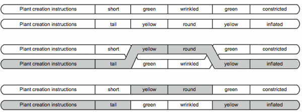
Fig. 4. A diploid pairing before, during, and after crossover.
Variation and stasis
As we discussed in the section on the random sequence model, stasis is very important and is clearly observable in nature. Although we observe wide and rapid variation within organisms of a given kind every day, observation also shows us that every child is the same kind as the parent.
From the discussion of sexual reproduction we can see how the computer program model supports simultaneous variation and stasis even though other models do not. Stasis is guaranteed, because the operational component (the instructions) does not vary. On the other hand, data is allowed to vary widely. Because each data segment has more than one value (or allele in biology) by definition, we can substitute any data segment for another of the same type and generate a great deal of variation without altering the definition of the kind at all. Computer programming languages very consciously use variables for the specific reason of supporting variation in output without altering the instructional code. By its very nature the computer program model solves the problem of simultaneous variation and stasis.
The computer program model explains why dog breeders, for example, can breed dogs to get all kinds variety, but have never made any steps toward a different kind of animal. Unlike any evolutionary model, which sees variation as modification of the genetic instructions, the computer program model sees breeding as simply shuffling the variable values within the population while leaving the instructional segments unchanged. No matter how much you shuffle a deck of cards, they are still cards. The game is not defined by what is on the cards, but by the rules. You can never alter the game by shuffling cards. To change the game someone has to create new rules. The hands will vary widely by shuffling, but the game will remain constant, because the instructions, or rules, are separate from the data, or cards.
Variation, mutation and the natural laws of information
Through the examples presented in this paper we have shown that the computer program model can explain variation without requiring a violation of the First Law of Information. This is because the computer program model explains variation as data substitution not as mutation of existing sequences. The instructional information and data were divinely created by God in the beginning (Genesis 1) and variation occurs by random substitution of variable values during inheritance. Variation is not an alteration of the operational information through mutation. No new information is created. The computer program model explains how the biblical revelation of created kinds is a better explanation of DNA than the evolutionary idea of common descent.
While the evolutionist world view sees mutations as the means of variation and change, the biblical world view sees mutations as part of the curse resulting from sin. (Note: In this discussion I am not classifying an alteration of DNA arising from healthy processes such as crossover as a mutation.) The Bible tells us that, because of Adam’s sin, the world is under a curse resulting in death (Genesis 3). From this we would expect that random natural forces could result in a loss of information, but not a gain. This is exactly what scientific research shows us regarding mutations, as Gitt shows when he says that, “. . . mutations can only cause changes in existing information. There can be no increase in information, and in general the results are injurious” (Gitt 2007, p. 126).
Spetner echoes this same idea when he says,
Not even one mutation has been observed that adds a little information to the genome. That surely shows that there are not the millions upon millions of potential mutations the theory demands. There may well not be any. The failure to observe even one mutation that adds information is more than just a failure to find support for the theory. It is evidence against the theory. We have here a serious challenge to neo-Darwinian theory (Spetner 1997, p. 160).
Rather than depending on mutations as an explanation for variation, the computer program model reflects the biblical view on mutations. As discussed before, if you mutate data you will get a new allele, but you will not get new functionality. The mutation may be beneficial in a localized environment, but it is never a gain of information. In most cases randomly mutating data will result in impaired output or even failure of the program, because the instructions cannot find the type of data it needs. Because instructional code must have specified complexity, if you randomly mutate instructional code, you will not get improved functionality. At best you will get impaired functionality. However, even the most novice programmer knows that if you randomly mutate instructional code, the overwhelming probability is that the functionality will fail altogether.
Biomorphs: A Summary of the Issue of Variation
Perhaps the most telling illustration of the lack of understanding of information models, as applied to the question of evolution, is found in Richard Dawkins’ biomorphs. We can use the biomorph program to summarize the points we’ve been making in this paper. A similar type of analysis could be done for any simulation of biology to see what kind of information model it uses.
Biomorphs are images created by a program Richard Dawkins wrote to illustrate evolution. In the program nine genes are simulated. By varying the value in the genes a huge variety of images can be created (Dawkins 1996). What is astounding is that Dawkins never understood what he did and did not demonstrate. It’s even more astounding that eminent thinkers, such as Steven Hawking, have referenced biomorphs in their own work as illustrations of the power of evolution without realizing that biomorphs strongly illustrate the viewpoint of the biblical creationist not the evolutionist (Hawking 2001)!
Dawkins is rightly amazed at the variety produced by his program, but to equate the variety with molecules-to-man evolution is to totally misunderstand the difference between information models that have variables and those that do not. Each gene in Dawkins’ program is a variable! Variables, by definition, are specifically designed to allow variation without evolving the program. No matter what the appearance, every biomorph created is of the same kind. Biomorphs are all static, symmetric, black and white, stick drawings with two branches at each node and a varying depth of recursion.
At least Dawkins is trying to model genes in DNA, but does this mean that all living organisms share the exact same chromosome map? All biomorphs do. The biomorph genome is only evolving in the sense that the variable values for the initial biomorph is not the same as the genome of any final biomorph, but this has everything to do with variation and nothing to do with common descent. Dawkins models his genome using the random sequence model and so it appears to him like evolution, because the sequence of symbols does not stay fixed. However, the reader should notice that the instructions to interpret the data never changes.
From the perspective of the computer program model, Dawkins left something very important out of the genome. He left out the instructional code that interprets the genes. So, his model for the genome is incomplete. Dawkins did not illustrate evolution, he illustrated the incredible variety that can exist within a single created kind, because they have the exact same set of genes and instructional code. The meaning of each variable is not determined by the data, which changes, but by the instructions, which do not change. What each of the nine genes stands for was totally and completely determined by the programmer. Those same nine genes could have been interpreted as something else if Dawkins had so written the program.
Dawkins speaks of “a version of the program that uses a few more ‘genes’ to control colour” so that “insects will actually cause the evolution, in the computer, of flowers” (Dawkins 1996, p. 63). I haven’t heard how that worked out for him, but the question is, why did he have to create a new version of the program to add new genes? As we have already discussed, mutations can give you new alleles, but not new genes. This is exactly the point of the discussions of specified complexity. You cannot randomly create information. This is why computer programs separate the instructions from the data. You can vary the data all you want and get very interesting results, but you will never get a better program by varying data.
Later on Dawkins laments a number of improvements he would like to see in his program, “I had no means of recording their genes” (Dawkins 1996, p. 64), and “I wanted to try to represent this genetic space in the form of a picture” (Dawkins 1996, p. 67), etc. If cumulative selection is so powerful, then why didn’t Dawkins use it to evolve the features he wanted, when he wanted them? If cumulative selection can create the sentence “METHINKS IT IS LIKE A WEASEL” in about 40 generations (Dawkins 1996) surely a few lines of code can be generated in a short time. But Dawkins’ answer to each of the programming problems is not to turn to cumulative selection and common descent, but to invoke a designer, because he, like any programmer, realizes that if you randomly mutate instruction code you get disaster, not a better program.
It is important for the reader to recognize that the computer program model is not about a particular computer program that implements evolution or simulates biology. Instead it is a proposal that computer programs themselves, along with an instance of data, are a type of information that we can use to model DNA. This is what Dawkins did not see. His genome was simply a sequence of random values, not a computer program with variables. The point is not what any particular program can do, but whether the system models the genome as instructions combined with data in the same stream.
Conclusion
In this paper we have seen that for a random sequence of symbols or a set of sentences variation occurs by mutating the existing sequence. This aligns with an evolutionary world view, but these models are not good models for DNA, because they cannot explain variation in light of stasis and the First Law of Information. On the other hand the computer program model explains variation by data substitution and forms an excellent model for DNA. We have seen that altering data in a computer program will never cause the program to evolve, because computer programs separate data from instructions by using variables. With the computer program model we can understand how wide variation can occur simultaneously with stasis and the First Law of Information is not violated.
The computer program model can also explain structures and patterns in DNA and leads us to a proposed informational definition of biblical kinds:
Biblical Kind—The set spanned by all organisms having the same instructional segments and structural arrangements in DNA.
From these findings we can conclude that equating externally observed differences with evolution is completely false, because it fails to recognize that variation can occur without any implication of evolution if the information system uses variables. A practical consequence is that the term “microevolution” should be strongly rejected along with any definition of evolution such as, “a process that results in heritable changes in a population spread over many generations” (Moran 1993) or “any change in the frequency of alleles within a gene pool from one generation to the next” (Curtis and Barnes 1989, p. 974).
These terms and definitions fail to understand that for any system that uses variables, variation has nothing to do with change in kind. Therefore they are clearly inappropriate and hinder scientific investigation. To be credible, future investigations of DNA must incorporate an accurate model of information. Such a model can help baraminological research (the study of created kinds) by providing a basis for recognizing the created kinds based on the structure of DNA. This paper proposes that the computer program model is currently the best model of information in DNA and hopefully helps provide a small step toward understanding the functional structure of DNA.
Because the computer program model agrees with the biblical record and forms a stronger basis for understanding biological variation than either a random sequence model or a sentence model, this paper concludes that the Bible provides a superior foundation for understanding variation within the living world. With regard to information, the Bible revealed to us over 3,500 years ago what we are just beginning to understand today. Differences in living organisms are constrained to variation within types or kinds. The biblical account even implies the most accurate information model, namely one that uses variables, if we had just known to look.
This paper has merely introduced the possibility that computer programs form a good model for understanding DNA. Areas of future research might begin by considering what control structures exist within portions of DNA that do not code for proteins. Is there a direct computer program analogy for hox genes? Are the structural arrangements of chromosomes simply organizational or do they affect control flow? Are there local variable equivalents that might be affected by environment? Could some segments be counters, limits, or addressing mechanisms?
Now is a perfect time for computer scientists to begin closely investigating the structure of DNA. Neither the biologist nor the engineer studies and creates informational structures on a daily basis, so the input of computer scientists can be invaluable. Let us abandon simplistic and inaccurate models and move to a clearer and stronger understanding of God’s wondrous creation that we might give honor to whom honor is due.
Psalm 139:14
I praise you because I am fearfully and wonderfully made; your works are wonderful, I know that full well.
References
Aho, A. V., R. Sethi, and J. D. Ullman. 1986. Compilers: Principles, techniques, and tools. Reading, Massachusetts: Addison-Wesley Publishing Company.
Ayala, F. J. 2009. Molecular evolution. In Evolution the first four billion years, eds. M. Ruse and J. Travis. Cambridge, Massachusetts: The Belknap Press of Harvard University Press.
Behe. M. J. 1996. Darwin’s black box: The biochemical challenge to evolution. New York: The Free Press.
Behe. M. J. 2007. The edge of evolution: The search for the limits of Darwinism. New York: The Free Press.
Bluedorn, N. and H. Bluedorn. 2003. The fallacy detective: Thirty-six lessons on how to recognize bad reasoning, 2nd ed. Muscatine, Iowa: Christian Logic.
Bodmer, W. and R. McKie. 1995. The book of man: The human genome project and the quest to discover our genetic heritage. New York: Scribner.
Bradley, W. L. and C. B. Thaxton. 1994. Information & the Origin of Life. In The creation hypothesis: Scientific evidence for an intelligent designer, ed. J. P. Moreland. Downers Grove, Illinois: InterVarsity Press.
Curtis, H. and N. S. Barnes. 1989. Biology, 5th ed., p.974. New York:Worth Publishers.
Dawkins, R. 1996. The blind watchmaker: Why the evidence of evolution reveals a universe without design. New York: W. W. Norton & Co.
Futuyma, D. J. 1986. Evolutionary biology, 2nd ed. Sunderland, Massachusetts: Sinauer Associates.
Gitt, W. 2007. In the beginning was information: A scientist explains the incredible design in nature. Green Forest, Arkansas: Master Books.
Gould, S. J. 2002. The structure of evolutionary theory. Cambridge, Massachusetts: The Belknap Press of Harvard University Press.
Hawking, S. 2001. Our future? Star trek or not?: How biological and electronic life will go on developing in complexity at an ever-increasing rate. In The universe in a nutshell,
pp. 155–171. New York: Bantam Books.
Lenski, R. E., C. Ofria, R. T. Pennock, and C. Adami. 2003. The evolutionary origin of complex features. Nature 423, no. 6936:139–144.
Lester, L. P., and Bohlin, R. G. 1989. The natural limits to biological change, 2nd ed. Dallas, Texas: Probe Books.
Lightner, J. K. 2008. Karyotype variability within the cattle monobaramin. Answers Research Journal 1:77–88. Retrieved from http://www.answersingenesis.org/articles/arj/v1/n1/karyotype-variability-cattle on February 12, 2011.
Mansfield, R. 2009. Programming: A beginner’s guide. New York: McGraw Hill.
Milner, R. 1990. The encyclopedia of evolution: Humanity’s search for its origins. New York, New York: Facts On File.
Moran, L. 1993. What is evolution? Retrieved from http://www.talkorigins.org/faqs/evolution-definition.html on November 21, 2010.
Palladino, M. A. 2006. Understanding the human genome project, 2nd ed. San Francisco: Benjamin Cummings.
Parker, G. 2006. Darwin and biologic change. In Creation facts of life, pp. 75–147. Green Forest, Arkansas: Master Books.
Patterson, R. 2006. Evolution exposed: Your evolution answer book for the classroom. Hebron, Kentucky: Answers in Genesis.
Perry, G. 1993. Absolute beginner’s guide to programming. Carmel, Indiana: Sams Publishing.
Riddle, M. 2009. Information: Evidence for a creator? In The New Answers Book 2, ed. K. Ham, pp. 195–206. Green Forest, Arkansas: Master Books.
Ruse, M. and J. Travis, eds. 2009. Evolution the first four billion years. Cambridge, Massachusetts: The Belknap Press of Harvard University Press.
Silvertown, J. 2009. 99% APE: How evolution adds up. Chicago: The University of Chicago Press.
Spetner, L. 1997. Not by chance: Shattering the modern theory of evolution. Brooklyn, New York: The Judaica Press.
Travis, J. and D. N. Reznick. 2009. Adaptation. In Evolution the first four billion years, eds. M. Ruse and J. Travis. Cambridge, Massachusetts: The Belknap Press of Harvard University Press.
Wells, J. 2002. Icons of evolution: Science or myth?: Why much of what we teach about evolution is wrong. Washington, DC: Regnery Publishing.
Whitfield, P. 1993. From so simple a beginning: The book of evolution. New York: Macmillan.
Willett, E. 2005. Genetics demystified. New York: McGraw-Hill.


