Testing the Predictions of the Young-Earth Y Chromosome Molecular Clock: Population Growth Curves Confirm the Recent Origin of Human Y Chromosome Differences

Introduction

Young-earth creation (YEC) and evolution strongly disagree on the total timescale for human origins. Evolutionists stretch human history over 250,000 years (Karmin et al. 2015). In contrast, YE creationists put the origin of Adam and Eve about 6,000 years ago, and the most recent common ancestors of the global human race about 4,500 years ago at the Flood (Hardy and Carter 2014).

Consequently, these two origins models also differ in their accounts of the history of human events, and of past population sizes. These differences are a secondary consequence of their prior disagreement on the total timescale. For example, with 250,000 years at their disposal, evolutionists postulate many more events in human history than YE creationists, who invoke only a few thousand years.

Nevertheless, these two models agree on the human events and population sizes for the most recent 3,000 years of history. This conclusion follows from a comparison of mainstream archaeology to the biblical record. For example, mainstream archaeology tends to accept the existence of King David around 1000 B.C. (Coogan 1998). This date is close to the best biblical estimates that we have for King David (Hardy and Carter 2014). Beyond 1000 B.C., however, these two models diverge. For example, mainstream archaeology disputes or rejects the existence of the Exodus of Israel from Egypt (Coogan 1998). Since the traditional YEC date for the Exodus is around 1400 to 1500 B.C. (Hardy and Carter 2014), human history prior to 1000 B.C. is a model-specific pursuit.

In sum, for most of human history, YEC and evolution sharply dispute the events and population sizes that characterize the past. But for the most recent three millennia, these two models agree. In other words, for the events and population sizes for the last three millennia, YEC and evolution agree on the facts but disagree on their relative timing—whether they represent the tail end of a long, 250,000-year history, or the majority of a 4,500-year post-Flood history.

The field of genetics directly impacts this disagreement. Family trees derived from genetic data are records of past population sizes (Hamilton 2009). The field of genetics can also record the echoes of past human events, such as the separation and migration of human populations (e.g., the forcible split among African populations during the Trans-Atlantic slave trade) as well as encounters between isolated populations (e.g., the Mongol invasion of Europe). These types of events leave a genetic signature in the form of genetic isolation between populations and in the form of genetic intermingling among populations, respectively. In other words, with respect to the relative timing of the events and population sizes of the last 3,000 years, genetics holds the potential to test the YEC and evolutionary predictions.

Several considerations narrow the genetic arenas in which we can test these predictions. For example, for certain genetic compartments, YEC and evolution disagree not only on the total timescale but also on the mechanism by which DNA differences arise. For biparentally-inherited DNA, the evolutionary model explains all DNA differences ultimately via mutation. In contrast, the YEC model explains the vast majority of biparentally-inherited DNA differences via fiat creation of heterozygosity within Adam and Eve (Jeanson and Lisle 2016; Sanford et al. 2018). Consequently, for most nuclear DNA differences, YEC and evolution produce different family trees.

Without a common family tree, YEC and evolution predictions about ancestral population sizes and events cannot be tested head-to-head. Testing a difference in relative timing of population sizes and events within a tree requires agreement on the overall sequence of events reflected in the structure of the tree. Absent this shared tree structure, simple testing of YEC and evolution predictions is not possible.

In contrast, uniparentally-inherited DNA is free of these concerns. Because mitochondrial DNA (mtDNA) and the Y chromosome are inherited from only one parent—mothers or fathers, respectively (rare biparental mtDNA inheritance exceptions notwithstanding (e.g., see Luo et al. 2018)), YEC and evolution agree on the mechanism by which modern mtDNA and Y chromosome differences arose among the global human population. Both models explain these differences via mutations since the beginning of the human race. Thus, both models produce the same family tree. Therefore, both mtDNA and the Y chromosome possess much greater potential for testing the YEC and evolutionary predictions about the relative timing of human events and past population sizes.

Practically, only one of these two uniparentally-inherited DNA compartments lends itself to useful inference of ancestral population sizes. For mtDNA, branch length variation is significant; the standard deviation can be up to 25% (Jeanson, unpublished data; see also the visual evidence for this in Supplemental fig. 1 in Jeanson 2016). Thus, trying to recover ancestral population sizes at specific points in time is challenging. High temporal precision is nearly impossible to achieve, which makes the resultant inferences of ancestral population sizes of little use.

In contrast, the variation among branch lengths in trees derived from high coverage Y chromosome sequences is low—the standard deviation is on the order of 4% or less (see Supplemental table 11 in the accompanying Jeanson and Holland (2019) paper). When inferring ancestral population sizes at specific time points, this allows for high temporal precision.

To date, only one published, high sequencing coverage Y chromosome study has attempted to infer ancestral population sizes from the global human Y chromosome phylogenetic tree (Karmin et al. 2015). Karmin et al. (2015) performed their analysis within the 250,000-year framework of evolutionary time.

In Figure S4A of Karmin et al. (2015), the authors depicted their inferences of ancestral human population sizes for 8 different regional populations. Of the 8 studied populations, archaeological and historical data indicate that 7 have undergone a recent population spike (McEvedy and Jones 1978). One of the populations—the Native Americans— are known to have undergone a recent, massive population collapse (Denevan 1992; Mann 2005).

As visual inspection of Figure S4A of Karmin et al. (2015) reveals, the authors successfully detected population decline in the native Andean population. However, for the remaining seven populations, they failed to detect the recent spike in human population growth 70% of the time; they inferred a spike for only 2 of the 7 populations known to have undergone one.

Why has mainstream evolutionary science largely failed to detect recent population growth—let alone place it at the tips of the tree? In the accompanying paper (Jeanson and Holland 2019), we found that the Y chromosome mutation rate was much higher than that which the evolutionary model predicted. This implied that the total timescale for the human Y chromosome tree was only a few thousand years, rather than the ancient timescale adopted by Karmin et al. (2015). Furthermore, the actual mutation rate appeared to be 2 to 3 base pairs per generation, on average. A rate this high implied very fine temporal resolution for the derived family tree of humanity, and it gave added to significance to each branch on the tree. In other words, the fact that mutations occurred every generation implied that the Y chromosome could record changes in human population size at every generation in human history. Perhaps the low mutation rate accepted by Karmin et al. (2015)—and resultant implications for the significance (or lack thereof) for each branch in the Y chromosome tree—led to their failure to detect the recent spike in human population growth in the majority of their tests.

Regardless of why Karmin et al. (2015) failed, the YEC hypotheses on the relative timing of the events and population sizes of the last 3,000 years remain untested. In this paper, I tested these predictions with the primary data from Karmin et al. (2015). Specifically, I tested whether the ancestral human population sizes of the last 3,000 years matched the inferred population growth from the tips of the Y chromosome tree, or from both the tips and many of the internal branches of the Y chromosome tree. The YEC timescale predicts a match to the latter.

The initial results that I uncovered in this study led me to explore additional facets of human origins. Because my results confirmed the YEC timescale so strongly (see below), I explored the YEC implications more deeply. For example, no published YEC study has positively identified where the “Noah” position (i.e., the actual root) in the Y chromosome tree exists. I used my population growth results to inform this question. Conversely, the reliability and implications of ancient DNA—such as that obtained from Neanderthal bones—remain contentious, both among YE creationists (Jeanson 2015; Wood 2012, 2013), and between evolutionists and YE creationists (Frello 2017a, 2017b; Jeanson 2017a, 2017b). I used my population growth results to test various hypotheses on Neanderthal DNA.

Materials and Methods

Y chromosome trees

I utilized two types of Y chromosome phylogenetic tree data from Karmin et al. (2015). The first type of data was taken from their Figure S3 and from their Table S7, which lists all the branch points and associated time values. The second type was derived from their accompanying primary data in their online VCF file, which I converted to FASTA form, and then used the FASTA file to draw a neighbor-joining tree (see accompanying Jeanson and Holland 2019 paper for details and references on how I derived the tree from the VCF file).

Population growth inference

The findings of the accompanying paper (Jeanson and Holland 2019) indicated that the per-generation Y chromosome mutation rate was 2 to 3 base pairs per generation. Implicitly, this suggested that the Y chromosome could record every new branch that formed over time—and that simply counting the accumulation of Y chromosome branches over time would reflect changes in ancestral human population sizes. I applied this suggestion to the design of my population size inference methods.

Published tree

The published tree in Figure S3 and in Table S7 of Karmin et al. (2015) does not report branch lengths in units of base pairs but, rather, in units of (evolutionary) time. Since I was testing the predictions of the YEC timescale, I treated the units of (evolutionary) time as surrogate/relative markers of molecular distance, which then would ultimately be converted back to units of calendar time.

For example, in their published tree (their Figure S3), we know that node 5 is a certain molecular distance away from the tips of the tree for individuals in haplogroup C and in haplogroups G through T. However, in Table S7 of Karmin et al. (2015), the average molecular “distance” is reported as 71,048 years before present; it’s not reported in units of base pairs. Nevertheless, I simply treated years before present as a relative marker of base pair distance, which I later converted back to units of calendar time.

Practically, this approach played out in the following manner: First, I chose a root position for the tree. At first, I simply adopted the root position accepted by Karmin et al. (2015); subsequently (see below), I tested alternative root positions. Second, the years before present distance—i.e., my surrogate for actual base pair distance—from this root to the tips of the tree (“root-to-tip” or “R2T”) was divided into the YEC post-Flood timescale (see accompanying Jeanson and Holland 2019 paper for a derivation of this range of values). In this paper, I treated the post- Flood timescale (“PFT”) as 4,206 to 4,636 years long. Third, a “present” calendar year (“PCY”) was chosen (either 1950 or 1990—see Jeanson and Holland 2019 paper for justification). Fourth, since years before present for each branch point node is a surrogate marker for actual base pair distance from each PCY (i.e., tip) to each branch point node, I treated each tip-to-node (“T2N”) years before present quantity as a relative marker of molecular distance.

Fifth, I converted the years before present quantity for each branch point node into a calendar date with the following equation:

Calendar year for population splitting (growth) event = PCY – (T2N / (R2T / PFT))    (1)

To account for inherent error in the construction of the Y chromosome tree, I utilized the published error reported in Table S7 of Karmin et al. (2015). Specifically, I transformed the reported “Lower^a” and “Upper^a” values for root positions (or early sub-root positions; see Supplemental tables 1–5 for details) by dividing the “years before present” value by one of the PFT values. Then I divided each reported T2N distance—including the average, “Lower^a”, and “Upper^a” values for these T2N distances—by these converted R2T values. To keep the math simple, I divided similar data into one another—i.e., “Lower^a” T2N into “Lower^a” R2T; “Upper^a” T2N into “Upper^a” R2T; average T2N into average R2T. I then subtracted the result from one of the PCY values.

After performing these calculations, maximum and minimum dates were identified for each branch point.

After performing these calculations for all branch points, the time points were then sorted by date, and then plotted sequentially. Time points for minimum values were sorted by date and kept separate from time points for maximum values, which were also sorted independently by date. For simplicity of viewing, B.C. calendar dates in my figures were treated as negative numbers; A.D. dates, as positive numbers.

These results were then compared to the shape of known global population growth on a dual-y-axis graph (see Supplemental tables 1–5 for details). World population values were obtained primarily from McEvedy and Jones (1978). Reported population sizes for regions and for the entire globe were converted to male-only population sizes by dividing the reported population size by 2. Population values were also obtained from Appendix B of Maddison (2001). I used the McEvedy and Jones (1978) dataset for my minimum values [it was the minimum value— or close to it—in the Maddison datasets], and then took the maximum values from Maddison (2001).

The Maddison (2001) and McEvedy and Jones (1978) datasets differed in ways that required extrapolation to make the two comparable. For example, the McEvedy and Jones (1978) data have more temporal detail—i.e., Maddison reports world population sizes for only the B.C./A.D. transition, for A.D. 1000, for A.D. 1500, and for A.D. 1700, whereas McEvedy and Jones (1978) report world population sizes generally every 100 to 200 years throughout the last three millennia, with even smaller time intervals near the present.

To make the two datasets more comparable, I estimated maximum population values for McEvedy and Jones time intervals where Maddison did not report a value. I did so by extrapolating from the fold-difference between the two datasets on dates where they both reported population sizes (see Supplemental table 6 for details). For example, the minimum/maximum difference for the year A.D. 1700 was 1.11-fold different between the two datasets. For the 50-year to 100-year intervals that McEvedy and Jones (1978) reported but Maddison (2001) did not pre-A.D. 1700, I took the McEvedy and Jones values and multiplied them by 1.11 until the values for the year A.D. 1500 were reached.

As another example, in the year A.D. 1500, the reported Maddison value was 1.14-fold higher than the reported McEvedy and Jones value. Thus, for the McEvedy and Jones values for the year A.D. 1500, I multiplied them by 1.14, as well as for all their reported values back to just before the year A.D. 1000.

For the year A.D. 1000, the Maddison values were 1.17-fold higher than the McEvedy and Jones values. Thus, from A.D. 1000, I multiplied the McEvedy and Jones values by 1.17, as well as for all their reported values back until just before A.D. 1.

For A.D. 1, the fold-difference between the datasets was 1.74-fold. For McEvedy and Jones values for A.D. 1 and earlier, I multiplied them by 1.74.

Of the available estimates of historical population sizes, Maddison (2001) and McEvedy and Jones (1978) represent much of the spectrum of historical population estimates (see this site1 for range of comparisons), which can vary widely—both in magnitude and direction, and differently for different time points (i.e., one source might represent the high estimate for an early time point, and a low estimate for a recent time point).

Before comparing these historical data to the population growth curves inferred from the Y chromosome, I added a correction factor to the historical data. My reasoning was as follows: Because Karmin et al. (2015) sampled living males, they effectively sampled the history of only those historical lineages that left survivors in the present. From historical records as well as from archaeology, it is well known that the last 3,000 years of human history record periodic population downturns and episodes of population stasis (i.e., see McEvedy and Jones 1978). Population downturns imply loss of Y chromosome lineages, due to death of male offspring or, simply, to failure to reproduce. Similarly, population stasis can lead to loss of lineages. For example, Biggar et al. (1999) contains an analysis of over 700,000 Danish families at population stasis (i.e., number of children born was equivalent to the sum of the number of fathers and mothers). Their results showed that 28% of fathers left no male offspring (see Table 1 of Biggar et al.). Thus, by sampling the historical male lineages that survived, no one using Karmin et al. (2015) data would ever be able derive a population growth event followed by a downturn. Rather, inferences derived from Karmin et al. (2015) data would simply depict the lineages that made it through the downturn.

Thus, to make the evaluation of my predictions more rigorous, I converted the known global population growth curves from Maddison (2001) and McEvedy and Jones (1978) into minimum population growth curves. Where historical stasis or downturn events occurred, I connected the growth curve data points at their minimum values. Practically, this resulting curve is a type of smoothed global population curve (Supplemental fig. 1; see also Supplemental table 6).

Because my results contained uncertainties in the range of hundreds of years, I did not bother to correct my time scales for absence of a “year zero” (i.e., the abrupt transition from 1 B.C. to A.D. 1).

Derived tree

I used my derived neighbor-joining tree (see Supplemental fig. 3 of Jeanson and Holland 2019) as a secondary confirmation of the findings from the published tree. In this derived tree, I calculated calendar dates for each branch point using the base pair distances depicted on this tree. Practically, my approach played out similar to the approach I employed for the published tree, with slight changes: First, I chose a root position for the tree. At first, I simply adopted the typical evolutionary root position; subsequently, I tested the “Alpha” root position (see definition below). Second, the actual base pair distance from this root to each branch tip (“root-to-tip” or “R2T”) was calculated. Third, I identified the YEC post-Flood timescale (see accompanying Jeanson and Holland 2019 paper for a derivation of this range of values). In this paper, I treated the post-Flood timescale (“PFT”) as 4,206 to 4,636 years long. Fourth, a “present” calendar year (“PCY”) was chosen (either 1950 or 1990—see Jeanson and Holland 2019 paper for justification). Fifth, I counted the base pair distance from the root to each branch point node (“R2N”).

Sixth, I utilized all of these factors to determine calendar dates for each branch point node. Effectively, I treated molecular distances as surrogates of time, and calculated a unitless time ratio with the R2T and R2N values, which I multiplied by the PFT. See the following equation:

Calendar year for population splitting (growth) event = PCY – (PFT – (R2N / R2T * PFT))    (2)

To account for inherent error in the construction of the Y chromosome tree, I performed this calculation for each node under values I defined as “maximum” and “minimum.” For all descendants of a particular branch point node, I found the maximum R2T distance and the minimum R2T distance, and calculated calendar dates for each branch point node under both of these R2T distances with equation 2 above.

After performing these calculations for all branch points, the time points were then sorted by date, and then plotted sequentially. Time points for minimum values were sorted by date and kept separate from time points for maximum values, which were also sorted independently by date. For simplicity of viewing, B.C. calendar dates in my figures were treated as negative numbers; A.D. dates, as positive numbers.

These results were then compared to the shape of known global population growth on a dual-y-axis graph (see Supplemental tables 7–8 for details). World population values were obtained and used as above for the analyses of the published tree.

Again, because my results contained uncertainties in the range of hundreds of years, I did not bother to correct my time scales for absence of a “year zero” (i.e., the abrupt transition from 1 B.C. to A.D. 1).

Quantification of matching

The percent match between the YEC-based inferences of ancestral population sizes and the known historical population sizes post-1000 B.C. were quantified visually (see Supplemental tables 1–5, 7–8 for details). A match was defined as a state in which one or more of the blue lines (i.e., inferred population size) fell on or between the black lines (i.e., known population size). Mismatches were defined as a state in which neither of the blue lines (i.e., inferred population size) fell on or between the black lines (i.e., known population size). The amount of calendar years from the blue lines that matched or mismatch the black lines was set over the total timescale of analysis (i.e., 2,975 years, or the time from 1000 B.C. to A.D. 1975; A.D. 1975 was chosen because it is the last reported year in McEvedy and Jones (1978)).

Definition of roots

For the published tree

The “Evo” root was defined as node 1 in Figure S3 and Table S7 of Karmin et al. (2015). The Neanderthal root was defined as node 1 of Karmin et al. (2015)— but effectively with a years before present distance that was twice as many units as those reported in Table S7 (see Supplemental table 2 for details).

For alternate root positions, I used two types of mutually exclusive criteria to identify a range of candidates. The first criterion attempted to optimize the detection of triad-like structures near the root, as well as ethnically diverse lineages near the root. The pursuit of triad-like structures arose from the hypothesis that all three sons of Noah—Shem, Ham, and Japheth—would have left male descendants that would be easily identified today by a small but global sampling of male Y chromosome lineages. Conversely, the pursuit of ethnically diverse lineages arose from the hypothesis that many of the lineages in Genesis 10 (who descended from Shem, Ham, and Japheth) would have left male descendants that would be easily identified today by a small but global sampling of male Y chromosome lineages.

The second criterion attempted to mathematically optimize the orientation of the population growth curve. Biblically, the male post-Flood population began with just 4 men (Noah, Shem, Ham, Japheth), yet by 1975 (i.e., the final date given in McEvedy and Jones (1978)), the population had grown to nearly 2 billion. Practically, mathematical optimization would produce a tree orientation that put the fewest number of lineages near the root and the largest number of lineages at the tips. Thus, almost by definition, this mathematical optimization method avoided the pursuit of triad-like structures and the pursuit of a maximum of early, ethnically diverse lineages—since both pursuits would have inflated the number of early lineages and skewed the early-versus-late math ratios.

Deeper consideration of the multiplicative nature of human population growth further refined this criterion. Mathematically, biblical population growth of males spanned about 9 orders of magnitude— growing from an initial population of 4 men (e.g., Noah, Shem, Ham, Japheth) to nearly 2 billion in 1975. Yet the high coverage dataset that I employed (Karmin et al. 2015) spanned only 2 orders of magnitude (i.e., less than 350 men were sampled). Mathematically, it would seem unlikely that a sample of a few hundred men in the present would permit access to the entire population history of the globe.

Instead, under the second criterion, we might have expected these datasets to capture the most recent 3,000 years of human population growth. For example, in 1000 B.C., the male population was already 25 million. By 1975, this number had grown by only 2 orders of magnitude—to nearly 2 billion. Since the Karmin et al. (2015) dataset represented men sampled in the present and, therefore, represented a look back in time at the population growth that led to these living males, we might have predicted this approach to capture population growth post-1000 B.C. Before 1000 B.C., population sizes would have grown by 7 orders of magnitude—too great a change to be detected by our methods. Thus, we might have expected pre-1000 B.C. population inferences to be a flat line—no branching events due to the multiplicative nature of human population growth.

These two types of criteria were largely mutually exclusive because of their approaches to the math of population growth. The first type of criteria assumed that human male populations have been isolated since the Flood or since Babel to such an extent that the math of early human population growth post-Flood was irrelevant. So long as the choice of ethnolinguistic groups was sufficiently diverse, the earliest post-Flood history could have been accessed. In contrast, the second type of criteria treated the isolation (or lack thereof) among ethnolinguistic groups as irrelevant and placed the primary emphasis on the dramatic multiplicative increase in humanity since the Flood. In other words, the second criterion implicitly assumed that the earliest post-Flood history had been obscured by subsequent migrations, conquests, and unequal population expansions across diverse Genesis 10 lineages.

Applying these considerations to the Y chromosome tree in Figure S3 of Karmin et al. (2015), I observed that the Y chromosome tree possessed a type of triad structure near the junction of the haplogroup C lineages with the haplogroup A/B/D/E lineages and with the haplogroup F-through-T lineages (i.e., node 5 in Figure S3 of Karmin et al. 2015). This structure did not appear to be an artifact of the Karmin et al. (2015) analysis as it was also present in the 1000 Genomes Project data (see Supplementary Figure 14 of Poznik et al. (2016), especially node 72 on page 16 of the Supplementary Information). Hence, I inferred population growth curves (see Supplemental table 3 for details) from this root (hereafter, the “Gamma” root).

I also observed that a large number of geographically and ethnically diverse lineages joined where haplogroups F through T come together. In addition, a type of triad structure existed near the center of this junction (i.e., node 8 in Figure S3 of Karmin et al. 2015). This structure did not appear to be an artifact of the Karmin et al. (2015) analysis as it also appeared to be present in the 1000 Genomes Project data (see Supplementary Figure 14 of Poznik et al. (2016), especially node 258 on page 18 of the Supplementary Information). Hence, I inferred population growth curves (see Supplemental table 4 for details) from this root (hereafter, the “Epsilon” root).

However, because of Noah’s advanced age (500 years) at the begetting of his sons, he may have contributed an unusual number of mutations to his 3 boys (e.g., see Carter 2019; Carter, Lee, and Sanford 2018). Thus, I defined the Epsilon root more in terms of the positions of the 3 boys than in terms of the position of Noah. The 3 boys were defined as node 7, node 9, and part of the distance (defined in “years before present”) between nodes 8 and 193 (see Figure S3 and Table S7 of Karmin et al. 2015). Specifically, this latter position was defined by subtracting 1,465 “years before present” (treated as a distance, not a calendar date) from the given node 8 distance (i.e., measured in “years before present” in Table S7 of Karmin et al. 2015).

Finally, I observed that the Y chromosome tree contained a long, unbranching line close to the bullseye center of haplogroups C through T (i.e., the line between nodes 5 and 6 in Figure S3 of Karmin et al. 2015). This structure did not appear to be an artifact of the Karmin et al. (2015) analysis as it also appeared to be present in the 1000 Genomes Project data (see Supplementary Figure 14 of Poznik et al. (2016), especially the line connecting node 72 on page 16 of the Supplementary Information to node 168 on page 17 of the Supplementary Information). By the logic of the simple growth method, this unbranching line implied no (detectable) population growth. Conversely, known population growth from 1000 B.C. (e.g., 25 million men) to 1975 (around 2 billion men) represented a change in only 2 orders of magnitude, implying that the most significant differences in magnitude (about 7 orders) occurred pre-1000 B.C. Together, these observations suggested that the root might be near the center of the unbranching line that connected the junction of haplogroups A through E, to the junction of haplogroups F through T. Hence, I inferred population growth curves (see Supplemental table 5 for details) for this root (hereafter, the “Alpha” root).

For my derived tree

For my derived neighbor-joining tree (see Supplemental fig. 3 of Jeanson and Holland 2019), I sought to confirm the main findings of my analyses of the published tree. Hence, I tested population growth from only two root positions. I defined the “Evo” root as left-most split position (effectively, the midpoint root; it connects node 303 and node 298) in the tree, and I defined the “Alpha” root as the point halfway (i.e., 62 base pairs, or half of 124 base pairs) between nodes 483 and 511. See Supplemental tables 7–8 for more details.

Effects of sampling

I sought to explore the effects of sampling on the population growth curves inferred from the published Y chromosome tree from Karmin et al. (2015). To this end, I isolated/created subtrees from their published Figure S3 tree. For simplicity, I limited my analysis to subtrees based on the Alpha root position.

Specifically, I parsed the published tree into nodes that led to “terminal” branches and those that did not. I defined branches which had no additional branches splitting from them as “terminal” branches. I defined a “terminal” node as one that spawned a “terminal” branch.

Once identified, these “terminal nodes” were further divided based on sampling strategy. I defined these addition subcategories based on whether the individual at the tip of the terminal branch was from a group with a single sampled individual; or from a group with two sampled individuals; or from a group with three sampled individuals; etc. all the way to twelve sampled individuals (see Supplemental table 9, which is a curated version of Table S1 from Karmin et al. (2015)). For example, in Figure S3 of Karmin et al. (2015), node 275 in the tree leads to two terminal branches. The tips of each of these two branches are occupied by Buryat man. The Buryats were sampled 12 times in the Karmin et al. (2015) study. As another example, in the same Figure S3, node 76 also leads to two terminal branches. The first branch leads to a Mordvin individual, and Mordvins were sampled 3 times in the Karmin et al. (2015) study. The second branch leads to a French individual, and he is the only French man in the Karmin et al. (2015) study.

After classifying and partitioning all terminal nodes by sampling strategy, I then obtained the inferred dates for each node from the Alpha root-based population growth curve analysis (i.e., as given in Supplemental Table 5). Next, I sorted dates within each sampling group from oldest to youngest. I then plotted these growth curves against the known population history of the globe (see description in earlier section above) on a dual-y-axis graph. In each graph for each sampling strategy, I kept constant the range of values on the known population history y axis. This was done to make visual comparison of the inferred population growth curves more straightforward across the various graphs. See Supplemental table 10 for details and specifics on the terminal nodes and terminal branches.

For nodes that spawned two terminal individuals (i.e., nodes near the tips of the tree), I effectively counted each node twice—once for each individual descendant. Some nodes appeared in different graphs. For example, for terminal nodes that spawned terminal branches of men from different population sampling groups, the terminal node would appear in the graphs for each sampling group. Sometimes the same node appeared twice in the same graph, if both terminal individuals were part of the same sampling group.

Results

YEC Evo root captures 27% of recent pop growth

The population growth curve inferred from the Y chromosome based on the Evo root successfully captured the recent spike in human population growth (fig. 1; Supplemental table 1). However, it failed to capture the shape of population growth pre-A.D. 1150 (fig. 1; Supplemental table 1). In other words, the Y chromosome curve based on the Evo root captured only 27% of the history of global male population growth (fig. 1).

Fig. 1. “Evo” root and young-earth timescale capture over one quarter of historical population growth. Using the branch counting method and the Karmin et al. (2015) dataset, ancestral population changes were inferred from the Y chromosome tree, assuming a young-earth creation (YEC) timescale and the “Evo” position for the root. The range of these inferences (double blue lines) was compared to the smoothed shape of historical population growth, depicted in double black lines. About 27% of the historical growth was captured by the curve inferred from the Y chromosome. Negative numbers are used for B.C. years. Inferences from the Y chromosome and historical population growth were plotted on the same x axis, but differing y axes.

YEC Neanderthal root captures 14% of recent pop growth

I explored whether the addition of (theoretical) Neanderthal DNA sequences would improve the results of this analysis (see Supplemental table 2 for details). While high quality Y chromosome sequences from Neanderthals are not yet published, the preliminary data that we do possess (Mendez et al. 2016) suggests that Neanderthal DNA is more divergent from modern human Y chromosome sequences than any two modern sequences are from one another. Furthermore, in the Y chromosome tree, these divergent Neanderthal sequences appear to branch off haplogroup A lineages. In other words, addition of Neanderthal sequences would appear to root the tree similarly to the traditional Evo root—but with an even longer lag between the root and the diversification of additional Y chromosome haplogroups.

Not surprisingly, the amount of matching between the theoretical Neanderthal root-based population growth curve and the smoothed historical population growth curve was even poorer than the Evo root-based curve alone. After A.D. 1550, the curve closely matched the known smoothed population history (fig. 2; Supplemental table 2). However, prior to A.D. 1550, the two curves were far apart. In other words, the Y chromosome curve based on the Neanderthal root captured only 14% of the history of global male population growth (fig. 2).

Fig. 2. Neanderthal root and young-earth timescale capture a fraction of historical population growth. Using the branch counting method and the Karmin et al. (2015) dataset, ancestral population changes were inferred from the Y chromosome tree, assuming a young-earth creation (YEC) timescale and the Neanderthal position for the root. The range of these inferences (double blue lines) was compared to the smoothed shape of historical population growth, depicted in double black lines. About 14% of the historical growth was captured by the curve inferred from the Y chromosome. Negative numbers are used for B.C. years. Inferences from the Y chromosome and historical population growth were plotted on the same x axis, but differing y axes.

YEC Gamma, Alpha, Epsilon roots capture over 90% of recent pop growth

Even though both the Evo root-based and Neanderthal root-based population growth curves manifested a recent spike as expected, the poor match between these curves and most of the rest of known recent population growth led me to explore the possibility of additional Y chromosome root positions. As per the descriptions supplied in the Materials and Methods, I tested the “Gamma”, “Epsilon”, and “Alpha” root positions.

Population growth inferences from all three of these root positions (Gamma, Epsilon, Alpha) captured the vast majority of the smoothed global population growth curve (figs. 3–5). Aside from the post-A.D. 1775 elements of the curves, and aside from minor deviations pre-A.D. 1775, the Y chromosome curves were a tight fit to the smoothed global population growth curve (figs. 3–5). These results were strong confirmation of the YEC population growth predictions, and they also suggested that the actual root was somewhere among these three root positions—if not identical to one of them.

Fig. 3. Gamma root and young-earth timescale capture vast majority of historical population growth. Using the branch counting method and the Karmin et al. (2015) dataset, ancestral population changes were inferred from the Y chromosome tree, assuming a young-earth creation (YEC) timescale and the Gamma position for the root. The range of these inferences (double blue lines) was compared to the smoothed shape of historical population growth, depicted in double black lines. About 90% of the historical growth was captured by the curve inferred from the Y chromosome. Negative numbers are used for B.C. years. Inferences from the Y chromosome and historical population growth were plotted on the same x axis, but differing y axes.

---

Fig. 4. Epsilon root and young-earth timescale capture vast majority of historical population growth. Using the branch counting method and the Karmin et al. (2015) dataset, ancestral population changes were inferred from the Y chromosome tree, assuming a young-earth creation (YEC) timescale and the Epsilon position for the root. The range of these inferences (double blue lines) was compared to the smoothed shape of historical population growth, depicted in double black lines. About 94% of the historical growth was captured by the curve inferred from the Y chromosome. Negative numbers are used for B.C. years. Inferences from the Y chromosome and historical population growth were plotted on the same x axis, but differing y axes.

---

Fig. 5. Alpha root and young-earth timescale capture vast majority of historical population growth. Using the branch counting method and the Karmin et al. (2015) dataset, ancestral population changes were inferred from the Y chromosome tree, assuming a young-earth creation (YEC) timescale and the Alpha position for the root. The range of these inferences (double blue lines) was compared to the smoothed shape of historical population growth, depicted in double black lines. About 95% of the historical growth was captured by the curve inferred from the Y chromosome. Negative numbers are used for B.C. years. Inferences from the Y chromosome and historical population growth were plotted on the same x axis, but differing y axes.

Replication of results with second tree

To test whether the results I observed with the published Karmin et al. (2015) tree were an artifact of their tree-building methodologies, I repeated my analyses with a tree I constructed from their VCF data (see Materials and Methods for details). Both the results based on the Evo root position (fig. 6) and the results based on the Alpha root position (fig. 7) matched the results I observed with these root positions in the published Karmin et al. (2015) tree (see figs. 1 and 5, respectively).

Fig. 6. “Evo” root and young-earth timescale capture over one quarter of historical population growth; derived tree. Using the branch counting method and my own tree derived from the Karmin et al. (2015) dataset, ancestral population changes were inferred from the Y chromosome tree, assuming a young-earth creation (YEC) timescale and the “Evo” position for the root. The range of these inferences (double blue lines) was compared to the smoothed shape of historical population growth, depicted in double black lines. About 31% of the historical growth was captured by the curve inferred from the Y chromosome. Negative numbers are used for B.C. years. Inferences from the Y chromosome and historical population growth were plotted on the same x axis, but differing y axes.

---

Fig. 7. Alpha root and young-earth timescale capture vast majority of historical population growth; derived tree. Using the branch counting method and my own tree derived from the Karmin et al. (2015) dataset, ancestral population changes were inferred from the Y chromosome tree, assuming a young-earth creation (YEC) timescale and the Alpha position for the root. The range of these inferences (double blue lines) was compared to the smoothed shape of historical population growth, depicted in double black lines. About 95% of the historical growth was captured by the curve inferred from the Y chromosome. Negative numbers are used for B.C. years. Inferences from the Y chromosome and historical population growth were plotted on the same x axis, but differing y axes.

Given these successful results, I did not perform any further tests with other root positions.

Can the mismatches be easily explained?

While the Gamma, Alpha, and Epsilon root positions captured more of the historical population growth curve than the Evo and Neanderthal root positions, none of the roots captured the entire history. I explored the implications of each root more deeply to understand whether the deviations from the historical growth curve were explicable under each hypothesis.

For each root, I explored two hypotheses on why each root position failed to capture the entire historical population growth curve. The first hypothesis posited that artifacts of sampling produced the mismatch between the two curves. In other words, to compare the Y chromosome curve to the historical global curve, the Y chromosome sequences must represent, as close as possible, a random sample of the globe. Any skewing or bias—such as might result from oversampling a region of the globe (e.g., a dataset consisting exclusively of German males) and undersampling others (e.g., a dataset that contains no Asian males)—would naturally produce deviations from the global historical curve. This first hypothesis suggested that sampling bias and skewing still exist in the current Y chromosome samples.

The second hypothesis posited that quirks arising from the known history of the globe have biased the Y chromosome sample. Under this hypothesis, sampling might have been statistically robust— with no oversampled or undersampled regions of the globe—but historical events might have led to the disappearance of historical populations. For example, among male Latin Americans, the main Native American haplogroup—haplogroup Q—is currently being outcompeted by European and African haplogroups. Over 75% of male Latin Americans do not fall in haplogroup Q (see Supplementary Table 9 of Poznik et al. (2016)); I also conducted my own unpublished analysis of Supplementary Figure 14 from Poznik et al. 2016). Since Europeans and Africans did not arrive in force in the New World until post-A.D. 1492, the drastic decline in haplogroup Q frequency occurred in just 500 years. If this population replacement continues unchecked, we might see the extinction of the Q lineage in the near future. Conversely, if this type of process occurred globally throughout history, then it may be impossible to access the earliest time points— because these early lineages might have been wiped out by later ones.

I first explored these two hypotheses in the context of the results based on the Evo root position. Based on the Evo root, the resultant growth curve implied that sampling before A.D. 1150 was poor (fig. 1). Furthermore, the sequence of events implied by the Evo root suggested that all non-African population growth began after A.D. 680 (i.e., see dates for node 4 in Supplemental table 1). In other words, either the sampling strategy failed to capture any pre-A.D. 680 lineages outside of Africa, or all pre-A.D. 680 lineages outside of Africa were wiped out by a post-A.D. 680 population group—a group that just happened to replace all lineages outside of Africa, from Papua New Guinea to Europe to Japan to the Americas. It’s difficult to find an event from known history that fits this explanation.

Thus, for the mismatch between the Evo root-based Y chromosome population growth curve and the historical population growth curve, the lack of plausible counter-explanations suggested that the mismatch represented real error—that the Evo root was not the actual root.

Alternatively, it might be possible to reconcile these mismatches with reality if Y chromosome mutation rates were higher in the past. This would effectively stretch the portion of the curve that matches over a longer period of history. However, a rough first approximation of this hypothesis was given by the Gamma-based root curve (see below). Given the parallel between the Gamma-based root hypothesis and the accelerated mutation hypothesis, I did not pursue the accelerated mutation rate hypothesis further.

For the Neanderthal root-based results, I found similar problems as those identified for the results based on the Evo root position. Based on the Neanderthal root, the resultant growth curve implied that sampling before A.D. 1550 was poor (fig. 2). Furthermore, the sequence of events implied by the Neanderthal root suggested that all non-African population growth began after A.D. 1300 (i.e., see dates for node 4 in Supplemental table 2). In other words, either the sampling strategy failed to capture any pre-A.D. 1300 lineages outside of Africa, or all pre- A.D. 1300 lineages outside of Africa were wiped out by a post-A.D. 1300 population group—a group that just happened to replace all lineages outside of Africa, from Papua New Guinea to Europe to Japan to the Americas. It’s difficult to find an event from known history that fits this explanation.

Thus, for the mismatch between the Neanderthal root-based Y chromosome population growth curve and the historical population growth curve, the lack of plausible counter-explanations suggested that the mismatch represented real error—that the Neanderthal root was not the actual root.

Again, because of the way the Gamma root (see below) approximated the accelerated past mutation rate hypothesis, I did not explore the possibility of faster past mutation rates.

For the Gamma, Epsilon, and Alpha roots, only a small section of mismatch required explanation. In general, all three roots tended to miss post-A.D. 1775 growth (figs. 3–5). Conversely, history seemed to be an unlikely explanation for this mismatch. Unlike the Evo and Neanderthal roots, none of these roots struggled to explain the origin of African or non- African sequences. All three roots placed the split between African and non-African lineages at the beginning or very near the beginning of post-Flood history. Also, nothing in the sequence of events implied by these three roots stood out as in egregious violation of the known historical sequence of events around the globe (see Supplemental tables 3–5 for details). For example, the implied sequence of events did not stipulate anything historically unsupported, such as an invasion of the United Kingdom within the last 200 years that led to the replacement of the population of the United Kingdom with peoples from Papua New Guinea.

In contrast, uneven global population sampling immediately suggested itself as an explanation for the mismatches. For example, the Karmin et al. (2015) dataset employed an inconsistent sampling strategy of the ethnolinguistic groups around the globe. Some ethnic groups were represented by a single male; others, by up to 12 males. Using the Alpha root-based results as a representative example, I found that the 1×-sampled populations gave population growth curves in fairly close alignment with known population history (fig. 8A; see Supplemental table 10 for details); all other sampling strategies resulted in lesser matches to known history—some of which were very poor matches (figs. 8B–J). As a general rule, I found that, the more highly-sampled the population, the more likely the growth curve was shifted disproportionately to the right side/more recent side of history (figs. 8B–J). In other words, more sampling of a given population led to increased detection of recent population growth. Together, these observations suggested that the mismatch post-A.D. 1775 for the Alpha root-based, Gamma root-based, and Epsilon root-based curves was likely due to unequal sampling of various ethnicities. It also predicted that even sampling of ethnicities would produce population growth curves with fewer mismatches. Conversely, it also predicted that heavy sampling of ethnolinguistic groups was essential to capturing the most recent population growth.

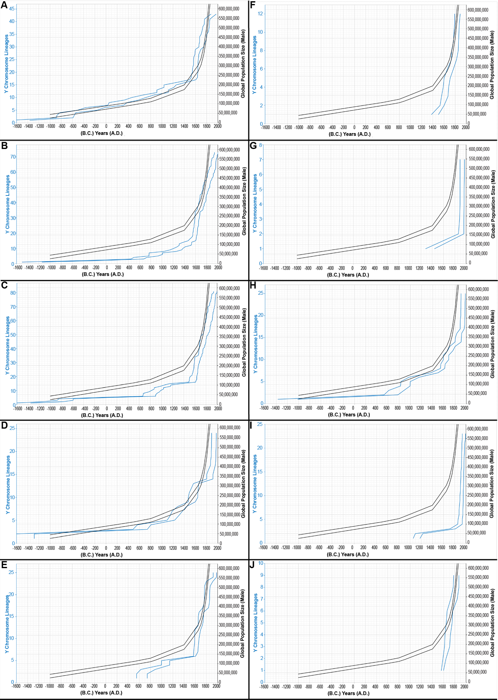
Fig. 8. Evidence for sampling errors. The inferred population growth curves, based on the Alpha root and on the young-earth creation (YEC) timescale, were re-drawn according to the number of times that a population was sampled. Rather than draw all branching events, only those leading immediately to a tip (without additional branching) were scored. Populations that were sampled one time (1×) are shown in (A); populations sampled 2×, in (B); 3×, in (C); 4×, in (D); 5×, in (E); 6×, in (F); 7×, in (G); 8×, in (H); 9×, in (I); 12×, in (J). Inferences from the Y chromosome and historical population growth were plotted on the same x axis, but differing y axes. The range of these inferences (double blue lines) was compared to the smoothed shape of historical population growth, depicted in double black lines to represent the range of historical estimates. The historical population size y axis was kept constant for sake of comparing the blue lines in (A)–(J). Inferences from the Y chromosome and historical population growth were plotted on the same x axis, but differing y axes. Negative numbers were used for B.C. years.

In sum, taking these observations together, my results suggested that the high levels of matching between the Alpha root-based, Gamma root-based, and Epsilon root-based population growth curves and the historical population growth curves were a result of the fact that these roots and the YEC timescale capture actual history.

Discussion

A test of the YEC timescale

The results in this paper represent an explicit test of the predictions of the YEC timescale. Conversely, the successful confirmation of this timescale represents one of the strongest scientific arguments in favor of it. The greatest strength of this argument derives from the scope of my methodologies. This scope is most easily seen by comparison. For example, pedigree-based mutation rate analyses (see accompanying Jeanson and Holland 2019 paper), while powerful, examine a much smaller window of history. By definition, father-son comparisons (or grandfather-grandson comparison) represent only the tips of the Y chromosome tree. The results of these tip analyses are then extrapolated backwards in time to test expectations of the evolutionary or YEC models. In contrast, my inferences of ancestral population sizes are based on the vast majority of the tree—not just the tips but also the internal branches. Thus, the strong confirmation of the YEC timescale across the vast majority of the Y chromosome tree makes counter-explanations from evolution all the more difficult to invoke.

Weighing evidence for specific YEC root positions

My positive results for the YEC timescale aid the search for the precise root of the Y chromosome tree. While my results strongly reject the traditional evolutionary and Neanderthal root positions, they do not yet give an exact position for Noah’s DNA sequence. For all three non-evolutionary, non- Neanderthal roots (e.g., Gamma, Epsilon, Alpha), the percent match between the inferred population history and the known population history was strong. Though the Alpha root resulted in the highest percent match in this dataset, the difference among the matching percentages for the Gamma, Epsilon, and Alpha roots was very small. Combined with the very small sample size of men in this dataset (i.e., as compared to the global male population), this small percent difference suggested than any of these three positions might be the actual Noah position.

Looking to the future, the best tests for Noah’s position will likely come from consideration of the earliest post-Flood time points. For example, visually, it is apparent that the biggest differences among the Gamma, Epsilon, and Alpha root positions are in the earliest time points (figs. 3–5). For instance, from ~2500 B.C. to 1000 B.C., the shape of population growth is very different for the Gamma-based versus Epsilon-based growth curves (i.e., compare figs. 3 and 4). Thus, scientifically, the clearest discrimination between these positions will come from tests that focus on these early time points.

These results should not be construed to claim that the Gamma, Epsilon, and Alpha root positions are the only plausible hypotheses going forward. Rather, these root positions define the most likely range of possibilities for the root—the range being anywhere on the branch connecting the Gamma and Epsilon root positions.

Conversely, it is also theoretically possible that Noah is still not yet depicted on our current trees. Mathematically, it seems very difficult to interrogate the earliest population changes that spanned 7 orders of magnitude. Our current population sampling might simply represent the most recent post-Flood history, with the earliest history still hidden among rare Y chromosome lineages yet to be discovered.

In summary, for future explorations of Y chromosome-based history, I recommend that investigators model at least the Epsilon and Gamma root positions when testing specific historical hypothesis, to avoid artificially biasing results in favor of a root position that may end up being wrong.

Biblical ramifications

If the subsequent investigations identify the Alpha root as the actual Noah position, this might reflect a typically overlooked biblical event. In Genesis 41, the text details Joseph’s interpretation of Pharaoh’s dreams and his subsequent promotion to second in command in Egypt. This chapter also describes Joseph’s preparation for the foretold famine, as well as the nations’ reliance on Egypt during the famine. Four times this chapter uses global-sounding statements to describe this event:

Then the seven years of plenty which were in the land of Egypt ended, and the seven years of famine began to come, as Joseph had said. The famine was in all lands, but in all the land of Egypt there was bread. So when all the land of Egypt was famished, the people cried to Pharaoh for bread. Then Pharaoh said to all the Egyptians, “Go to Joseph; whatever he says to you, do.” The famine was over all the face of the earth, and Joseph opened all the storehouses and sold to the Egyptians. And the famine became severe in the land of Egypt. So all countries came to Joseph in Egypt to buy grain, because the famine was severe in all lands. (v. 53–57, emphasis added; NKJV)

The surrounding biblical context for these verses lends support to the possibility that these statements are indeed speaking of the global humanity. For example, in Genesis 42, Jacob sends his sons to Egypt to gain relief from the famine. If the famine was local and not global, why not send his sons elsewhere, where bread could be found?

The date for this seemingly global famine and migration to Egypt can be derived from several statements in Scripture. Genesis 47:28 implies that Jacob was 130 years old when he entered Egypt. Conversely, Genesis 45:1–11 implies that he departed for Egypt at least two years into the famine. Given the dates for the patriarchs in earlier chapters in Genesis, we can put a calendar date on Jacob’s entry to Egypt, and then subtract two years to derive an estimate for a date for the start of the famine. With these data in hand (see Table 2 of Hardy and Carter 2014), the famine started anywhere from 620 to 699 years post-Flood. It lasted 7 years (see Genesis 41).

The sequence of events implied by the Alpha root-based inferences might reflect this biblical history. Under the Alpha root hypothesis, ethnic dispersal does not seem to happen near the Alpha root but later, after nodes 5 and 6 in Figure S3 of Karmin et al. (2015). The average date for these nodes is around 1830 B.C.—or about 620 years post-Flood, if we use 2450 B.C. as the average estimate for the start of post-Flood history. Conversely, the shape of population growth under the Alpha root hypothesis is also consistent with a famine happening about 620 years post-Flood. Before nodes 5 and 6 in Figure S3 of Karmin et al. (2015), little evidence for population growth exists, whereas population expansion happens thereafter. While this may reflect the mathematical sampling limits of the current study, it is also consistent with a famine-induced population downturn, followed by population regrowth post-famine.

Perhaps, after their migration to Egypt, people around the globe brought home more than bread.

Neanderthal DNA

My results further advance our understanding of the implications of DNA from Neanderthals—both for creationists and evolutionists. The strong match between my predictions (based on the Gamma, Alpha, and Epsilon root positions) and historical population growth is, itself, an argument against the reported—and very ancient—evolutionary geology-based dates for Neanderthal bones. If human history is as ancient as the evolutionists have claimed, we should not observe the strong matches throughout the Y chromosome tree that I observed in this study.

In addition, my results demonstrate the differences between Neanderthal DNA and modern human DNA is not an argument against the YEC timescale. Currently, the differences between Neanderthal DNA and modern human DNA is greater than the DNA difference between two modern humans (e.g., see an example from mtDNA in Jeanson (2015); see also Mendez et al. 2016). If Neanderthal DNA sequences are reliable, this might represent too great a difference to explain via constant mutation over 4,500 years. However, one indirect way to test the reliability of these sequences is to examine testable predictions that flow from this hypothesis. My results show that the hypothesis of reliable Neanderthal DNA sequences makes poor testable predictions. This is in contrast to those hypotheses that treat Neanderthal DNA as unreliable and modern DNA as reliable, which make successful population growth curve predictions.

With respect to the actual explanation for Neanderthal DNA differences, might Neanderthal DNA be reliable, but also the result of an accelerated mutation rate? My results suggest that this hypothesis is practically indistinguishable from the Gamma root position—which makes the Neanderthal-DNA-is-reliable hypothesis almost superfluous. Conversely, advocates of the accelerated mutation hypothesis will need to publish testable predictions that flow from this hypothesis, to distinguish it from the simpler hypotheses that the Gamma position is the actual root and that Neanderthal DNA is unreliable.

Testable predictions

The strong confirmation of the YEC timescale across much of the Y chromosome tree leads to additional testable hypotheses by which my model can be further examined. The simplest is a predictive mathematical formula for Y chromosome lineage discovery. This formula predicts the frequency with which deep-rooting Y chromosome lineages will be discovered in the future, and it derives from the multiplicative relationships among the known historical population sizes. As figs. 3–5 show, the multiplicative relationships among this historical population sizes match the multiplicative relationships among deep and shallow Y chromosome lineages. Thus, historical population sizes can be used to predict the discovery of deep Y chromosome lineages.

For example, in fig. 5, about 400 million men were alive around the years A.D. 1750 to A.D. 1800. From the inferred Y chromosome-based population growth curve, the number of Y chromosome lineages at that same time was about 225. In 700 B.C., about 50 million men were alive—an 8-fold reduction from 400 million. An 8-fold reduction from 225 Y chromosome lineages would be about 28 Y chromosome lineages. In 700 B.C., inferred Y chromosome-based population growth curve showed around 25—very close to the predicted 28.

As another example, consider the recent study of deep-rooting African lineages in haplogroup D (Haber et al. 2019). The authors state that these deep lineages were “first identified in 5 out of 1247 Nigerians” and “were subsequently reported in a single man among 282 from Guinea-Bissau in West Africa” (page 1422). These two latter discoveries were published in 2003 and 2007, respectively.

Haber et al. (2019) show that these deep lineages branch off the Y chromosome tree near where the D and E haplogroups join. Under the Gamma root hypothesis, this branch point (i.e., node 287 in Figure S3 of Karmin et al. (2015)) represents about 2210 B.C. Conversely, under the Epsilon root hypothesis, this branch point (i.e., node 287 in Figure S3 of Karmin et al. (2015)) represents about 1320 B.C.

Based on historical population growth in Africa, the multiplicative difference between the population size in A.D. 2003 and 1300 B.C. can be estimated. The male African population size in A.D. 2003 was around 436 million (see online United Nations data2). By 1000 B.C., the African male population was around 2 million (McEvedy and Jones 1978). Prior to 1000 B.C., it would have been even lower. (The YEC/evolution model-specific differences on pre-1000 B.C. human history make it difficult to determine an exact number for historical male African population sizes.) The multiplicative difference between A.D. 2003 and 1000 B.C. is 218-fold. For earlier dates, this fold-difference would be even larger.

Conversely, the multiplicative relationships from the Y chromosome discoveries mentioned in Haber et al. (2019) fit this relationship. For example, the number of recent lineages (i.e., 1247 Nigerians) is 250-fold higher than the number of ancient, deep-rooting haplogroup D lineages (i.e., 5). This is similar to the multiplicative relationship (i.e., 282-fold difference) between recent and ancient lineages for the men in Guinea-Bissau. Both of these values are close to the predicted fold-difference (i.e., >218-fold) from historical data.

As another arena of testable predictions, my results predict that the entire tree should reflect the known history of civilization post-1000 B.C.—not just the global history as a whole but also the history for specific subregions. Prior to 1000 B.C., human history is model-dependent, and, therefore, cannot be used as an independent test of my results. However, post- 1000 B.C., YEC and evolution largely agree on the specifics of human history. My results indicate that the Y chromosome tree should be consistent with this.

Specifically, for future exploration and testing, the most relevant historical data fall into a handful of categories. For example, where population growth and decline is known for specific regions of the globe, these data can be compared to the inferred population history from the Y chromosome. However, this test must be done in light of the caveats that constrain analysis of historical lineages from DNA obtained from the survivors. For instance, if the regional history is followed by an event where the indigenous population is destroyed or where it migrates away, these events must be accounted for by the methodology. Studies of the populations of the Americas represent a recent example of dramatic population changes and replacements (Denevan 1992; Mann 2005) where special caution is required.

Another type of relevant historical data is known population splits. For example, one of the most recent forced mass movements of peoples is the trans- Atlantic slave trade, for which very detailed historical information exists (e.g., see documentation online3). The Y chromosome split times between Africans and African Americans should be consistent with this known history. Specifically, the most relevant test will be the last cutoff point of the split—the point at which mixing ceased. For example, for dates after the slave trade was outlawed and effectively ceased, African and African-American lineages should not be joined—apart from more recent, non-slave trade migrations/immigration events. Prior to the slave trade stop date, coalescence between African and African-American Y chromosome lineages should follow the known history of population growth and decline in these populations.

Data quality

With respect to the results and conclusions in this paper, all are dependent on the levels of Y chromosome sequencing coverage. As the accompanying paper (Jeanson and Holland 2019) discusses and demonstrates, low coverage sequencing misses variants, including those in the tips of the tree. This will affect the inferred dates for population growth, population splits, etc. especially in the tips and less so in the deeper branches where the percent change in branch length will be less than in the tips. Since the analyses in this present paper are based on excessively filtered Y chromosome sequences (i.e., see Jeanson and Holland 2019), it’s likely that the specific calendar dates reported in this paper will be revised slightly when based on trees derived from better filtered Y chromosome data.

Also, the conclusions in this paper are based exclusively on the data from a single evolutionary publication. It will be important to see if these findings can be replicated with independent studies, especially those where special attention is paid to employing balanced sampling strategies.

Nevertheless, at present, my results represent a significant and strong advance for the YEC model, and a strong challenge to the evolutionary timescale.

It’s also remarkable that less than 350 men can reproduce the history of population growth over the last 3,000 years—and reproduce it to such high accuracy. This finding suggests that the Y chromosome tree may be a key tool for investigations of recent human history for years to come.

Acknowledgements

Special thanks to Rob Carter, for his helpful interactions over a period of many months, and for sharing unpublished data that helped spur the present analysis. Many thanks as well to the Answers in Genesis librarian, Walt Stumper, whose diligent efforts in tracking down sources—even if obscure—made the present paper possible. Thanks as well to Diane King for her help in file conversions of data in the Karmin et al. (2015) paper. Discussions of the biblical text were aided by Terry Mortenson and Matt Dawson. Reviewers of this work also helped refined and sharped the manuscript. One reviewer in particular supplied very helpful suggestions and critique.

References

Biggar, Robert J., Jan Wohlfahrt, Tine Westergaard, and Mads Melbye. 1999. “Sex Ratios, Family Size, and Birth Order.” American Journal of Epidemiology 150, no. 9 (1 November): 957–962.

Carter, Robert W. 2019. “Patriarchal Drive in the Early Post- Flood Population.” Journal of Creation 33, no. 1 (April): 110–118.

Carter, Robert W., Stephen S. Lee, and John C. Sanford. 2018. “An Overview of the Independent Histories of the Human Y-Chromosome and the Human Mitochondrial Chromosome.” In Proceedings of the Eighth International Conference on Creationism, 133–151. Edited by J. H. Whitmore. Pittsburgh, Pennsylvania: Creation Science Fellowship.

Coogan, Michael D. ed. 1998. The Oxford History of the Biblical World. New York: Oxford University Press.

Denevan, William M. ed. 1992. The Native Population of the Americas in 1492. Madison, Wisconsin: The University of Wisconsin Press.

Frello, Stefan. 2017a. “On the Creationist View on mtDNA.” Answers Research Journal 10 (August 23): 181–182. https:// answersingenesis.org/human-evolution/creationist-view-mtdna/.

Frello, Stefan. 2017b. “Reply to ‘Response to “On the Creationist View on mtDNA’”’.” Answers Research Journal 10 (October 4): 237. https://answersingenesis.org/human-evolution/reply-to-response-to-creationist-view-mtdna/.

Haber, Marc, Abigail L. Jones, Bruce A. Connell, Asan, Elena Arciero, Huanming Yang, Mark G. Thomas, Yali Xue, and Chris Tyler-Smith. et al. 2019. “A Rare Deep-Rooting D0 African Y-Chromosomal Haplogroup and Its Implications for the Expansion of Modern Humans Out of Africa.” Genetics 212, no. 4 (June): 1421–1428.

Hamilton, Matthew B. 2009. Population Genetics. Chichester, West Sussex, United Kingdom: Wiley-Blackwell.

Hardy, Chris, and Robert Carter. 2014. “The Biblical Minimum and Maximum Age of the Earth.” Journal of Creation 28, no. 2 (August): 89–96.

Jeanson, Nathaniel T. 2015. “Mitochondrial DNA Clocks Imply Linear Speciation Rates Within “Kinds.” Answers Research Journal 8 (June 3): 273–304. https://answersingenesis.org/ natural-selection/speciation/clocks-imply-linear-speciation-rates-within-kinds/.

Jeanson, Nathaniel T. 2016. “On the Origin of Human Mitochondrial DNA Differences, New Generation Time Data Both Suggest a Unified Young-Earth Creation Model and Challenge the Evolutionary Out-of-Africa Model.” Answers Research Journal 9 (April 27): 123–130. https://answersingenesis.org/genetics/mitochondrial-dna/origin-human-mitochondrial-dna-differences-new-generation-time-data-both-suggest-unified-young-earth/.

Jeanson, Nathaniel T. 2017a. “Response to ‘On the Creationist View on mtDNA’.” Answers Research Journal 10 (August 23): 183–186. https://answersingenesis.org/human-evolution/response-creationist-view-mtdna/.

Jeanson, Nathaniel T. 2017b. “Response to ‘Reply to “Response to ‘On the Creationist View on mtDNA’”’.” Answers Research Journal 10 (October 4): 239–240. https://answersingenesis. org/human-evolution/response-to-reply-to-response-to-creationist-view-mtdna/.

Jeanson, Nathaniel T., and Ashley D. Holland. 2019. Evidence for a human Y chromosome molecular clock: Pedigree-based mutation rates suggest a 4,500-year history for human paternal inheritance. Answers Research Journal 12: 393–404.

Jeanson, Nathaniel T., and Jason Lisle. 2016. “On the Origin of Eukaryotic Species’ Genotypic and Phenotypic Diversity: Genetic Clocks, Population Growth Curves, and Comparative Nuclear Genome Analyses Suggest Created Heterozygosity in Combination with Natural Processes as a Major Mechanism.” Answers Research Journal 9 (April 20): 81–122. https://answersingenesis.org/natural-selection/ speciation/on-the-origin-of-eukaryotic-species-genotypic-and-phenotypic-diversity/.

Karmin, Monika, Lauri Saag, Mário Vicente, Melissa A. Wilson Sayres, Mari Järve, Ulvi Gerst Talas, Siiri Rootsi, et al. 2015. “A Recent Bottleneck of Y Chromosome Diversity Coincides With a Global Change in Culture.” Genome Research 25, no. 4 (April): 459–466.

Luo, Shiyu, C. Alexander Valencia, Jinglan Zhang, Ni-Chung Lee, Jesse Slone, Baoheng Gui, Xinjian Wang, et al. 2018. “Biparental Inheritance of Mitochondrial DNA in Humans.” Proceedings of the National Academy of Sciences USA 115,no. 51 (December 18): 13039–13044.

Maddison, Angus. 2001. The World Economy: A Millennial Perspective (Development Centre Studies). Paris, France: Organization for Economic Cooperation and Development.

Mann, Charles C. 2005. 1491. New York: Alfred A. Knopf.

McEvedy, C., and R. Jones. 1978. Atlas of World Population History. Penguin Books, Middlesex, England.

Mendez, Fernando L., G. David Poznik, Sergi Castellano, and Carlos D. Bustamante. 2016. “The Divergence of Neandertal and Modern Human Y Chromosomes.” American Journal of Human Genetics 98, no. 4 (April): 728–734.

Poznik, G. David, Yali Sue, Fernando L. Mendez, Thomas F. Willems, Andrea Massaia, Melissa A. Wilson Sayres, Qasim Ayub, et al. 2016. “Punctuated Bursts in Human Male Demography Inferred From 1,244 Worldwide Y-Chromosome Sequences.” Nature Genetics 48, no. 6 (25 April): 593–599.

Sanford, John C., Robert W. Carter, Wes Brewer, John Baumgardner, and Bruce Potter. 2018. “Adam and Eve, Designed Diversity, and Allele Frequencies.” In Proceedings of the Eighth International Conference on Creationism, 200– 216. Edited by J. H. Whitmore. Pittsburgh, Pennsylvania: Creation Science Fellowship.

Wood, T. C. 2012. “Ancient mtDNA Implies a Nonconstant Molecular Clock in the Human Holobaramin.” Journal of Creation Theology and Science Series B: Life Sciences 2: 18–26.

Wood, Todd C. 2013. “Mitochondrial DNA Analysis of Three Terrestrial Mammal Baramins (Equidae, Felidae, and Canidae) Implies an Accelerated Mutation Rate Near the Time of the Flood.” In Proceedings of the Seventh International Conference on Creationism. Edited by M. Horstemeyer. Pittsburgh, Pennsylvania: Creation Science Fellowship.

Supplemental Files

Supplemental table 1.

Supplemental table 2.

Supplemental table 3.

Supplemental table 4.

Supplemental table 5.

Supplemental table 6.

Supplemental table 7.

Supplemental table 8.

Supplemental table 9.

Supplemental table 10.

Supplemental fig. 1. Estimates of recent human population growth. Over the last 3,000 years, human population growth has steadily risen, with a burst of growth in the last few hundred years. This latter spike in growth obscures the nuances of human population rises and declines in the years prior. Hence, the overall shape is depicted in (A), whereas (B) depicts the shape without the recent spike (compare y axes in (A) and (B)). Double lines (grey or black) represent the range of historical estimates. Grey lines represent actual history; black lines represent a smoothed version of the grey—they represent an estimate of what the growth curve for survivors of population downturns and of population stasis events looked like. Negative numbers are used for B.C. years.