
The views expressed in this paper are those of the writer(s) and are not necessarily those of the ARJ Editor or Answers in Genesis.
Abstract
The Genesis Flood must have produced drastic geological changes involving extremely energetic processes which must also have generated an enormous heat load. Yet since the inhabitants of the Ark and many aquatic creatures survived the Flood, the heat must have been removed without raising temperatures beyond biological endurance limits. This is the first in a series of papers intended to identify and, where possible, to quantify the most important sources of Flood heat. Here we review the thermal state of the earth’s mantle, crust and oceans, both now and in the recent geological past, and take note of mantle heterogeneities as tracers of its tectonic history. Extensive temperature records based on the oxygen-18 content of marine fossil shells indicate geologically recent ocean floor temperatures not exceeding 13ºC; all models of the Flood and its aftermath need to take this limit into account. A recent attempt to model ocean floor cooling within a biblical chronology by invoking a transient subsurface heat sink along with rapid oceanic plate movement was unsuccessful, suggesting that important hitherto-neglected geophysical effects may need to be included in future. Inventories of heat-producing radioactive elements estimated from rock compositions and from geoneutrino measurements are in broad agreement, lending confidence to the anticipated process of estimating the heat load due to accelerated nuclear decay during the Flood. Preliminary estimates for granite suggest that this radiogenic heat load would be overwhelming without the operation of a powerful in-situ cooling mechanism which has yet to be identified.
Keywords: mantle heterogeneities, temperatures, oxygen isotope palaeothermometry, oxygen-18, heat flow, radiogenic heat
Introduction
Chapters 7 and 8 of Genesis describe the catastrophic global Flood which God brought about at the time of Noah as judgment upon an incurably wicked human race and our environment. This Flood was of such scale and intensity that it must have drastically reshaped the face of the earth and deposited enormous quantities of heat. Since Noah, his family, the animals on the Ark, and many aquatic creatures survived the Flood, the atmosphere and oceans could not have been heated beyond biological endurance limits. The resulting scientific problem is to explain how the heat was removed without raising environmental temperatures too high.
This series of articles seeks to identify and, where possible, to quantify the sources of Flood-related heat in order to provide boundary conditions and guidelines for creation scientists seeking suitable explanations of how Flood and post-Flood environmental temperatures were kept within limits. Since some of the key background literature arises from the RATE (Radioisotopes and the Age of The Earth) project, the relevant RATE results are reassessed, partly to place on record an independent appraisal of RATE and some of the ensuing published exchanges
This article (Part 1) deals with boundary conditions relevant to modeling the earth’s thermal history. These include its internal temperature field, mantle structure, past and present ocean temperatures, surface heat flows and its inventory of heat-producing radionuclides. Given that several ocean temperature indicators are in current use, we focus here on ocean temperatures reconstructed from oxygen-18 data. Part 2 deals with newer, less familiar indicators including minor and trace element ratios, biomolecular indices and clumped isotopes. Part 3 reviews vapour canopy models, which are typically characterized by high pre-Flood atmospheric temperatures and a large heat load produced by collapse of the canopy at the beginning of the Flood. Part 4 assesses the heat released in Catastrophic Plate Tectonics (CPT), currently one of the most successful approaches to Flood modeling, and in similar Flood models; here the heat problem is caused by the large quantity of hot mantle material surfacing in a short time. Part 5 addresses probably the most acute Flood-related heat source, Accelerated Nuclear Decay (hereafter AND), which has been invoked to explain several key RATE findings; this heat source was recognized by the RATE authors (Vardiman et al. 2005). Part 5 also reassesses the methods and results of three components of RATE, viz. radiohalos in granites, fission tracks in zircons and helium diffusion in zircons.
Several authors have suggested that during the Flood the earth must have suffered a major bombardment from space; the resulting surface heat load is assessed in Part 6. Part 7 summarizes our conclusions and suggests possible directions for future investigations which might reveal a solution to Flood heat problems or to clarify key related questions.
Interior Temperatures and Structure of the Earth
Present-day conditions within the earth have been modeled using seismic, gravity, and geomagnetic data combined with compositional modeling of its constituent materials. Compositional models are informed by comparison with other bodies in the Solar System (sun, meteorites, and other planets). A representative model is the PREM (Preliminary Reference Earth Model) of Dziewonski and Anderson (1981); the data of interest here is conveniently summarized by Stacey and Davis (2008; Appendix F1 lists mechanical properties, Appendix G thermal properties). The resulting global averages as functions of distance r (in km) from the center of the earth are shown in fig. 1. The CMB (core-mantle boundary) shows its presence by a jump in temperature and a bend in the pressure profile, indicating a jump in density, at a depth of 2891km (r=3480km). Thermal boundary layers are evident (1) at the CMB, and (2) in the upper mantle between the transition zone (whose upper boundary is at a depth of 410km; see Frost 2008; Stacey and Davis 2008) and the surface. Such boundary layers are expected in the presence of the mantle convection associated with plate tectonic motions because there can be no advective heat transport through the CMB or through the lithosphere except at MORs and other localized volcanic outlets. The temperature drop through the region above the transition zone is approximately 1600K. The larger part of this occurs across the lithosphere, where also the temperature gradient is steepest; the thickness of the lithosphere, although very variable (Paysanos 2008), is typically of order 100km.
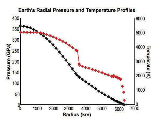
Fig. 1. Earth’s globally averaged internal pressures(black) and temperatures (red) as functions of radius (r),based on data from Stacey and Davis (2008).
Given spherically symmetric models of the kind proposed by Dziewonski and Anderson (1981) as a reference, geophysical evidence, mainly seismic, reveals considerable mantle heterogeneity (Kennett and Tkalčić 2008). The heterogeneity is especially pronounced in the D″ region, the lowest 200–300km immediately above the CMB, which is characterized seismically by a decreasing gradient of both P-wave and S-wave velocities with depth (Loper and Lay 1995). The heterogeneity is understood to be in temperature, composition, and material phase (Čížková et al. 2010; Hirose and Lay 2008; Klein,Jagoutz, and Behn 2017).
Regions of increased P- and S-wave speeds generally signify descending slabs, interpreted as subducted material, while lower wave speeds signify upwellings or mantle plumes. In many cases subducted material has apparently been flattened in the transition region around 660km below the surface (Fukao, Widiyantoro, and Obayashi 2001). However in the Farallon slab under North and Central America and the Indian/Tethys slab under the Himalayas and Bay of Bengal, subduction has reached the lower mantle. Baumgardner (2003) cites as evidence of mantle heterogeneity: (1) a ring of dense material at the bottom of the mantle, lying roughly below the perimeter of today’s Pacific Ocean; (2) superswells (e.g. in the South Pacific and under the East Africa Rift Valley), regions of locally elevated surface caused by rising mantle plumes (Grand, van der Hilst, and Widiyantoro 1997). Baumgardner (2003) cites density homogeneities up to the 3–4% level, and assuming this to be entirely thermal in origin, he infers temperature differences of up to 3000–4000K in the underlying mantle. He argues that differences this large are unlikely to have persisted for 100Ma (million years) as in the uniformitarian chronology, but are perfectly plausible if the subduction occurred only a few thousand years ago. However Baumgardner does not attempt to justify his assumption that compositional and phase-related contributions to density can be ignored.
Mantle heterogeneities, especially where they relate to subducted material, thus serve as an archive of earth’s tectonic history (Kennett and Tkalčić 2008). For example, a recent study has revealed, in uniformitarian terms, a link between the flux of subducted material reaching the CMB and the timing of geomagnetic field reversals (Hounslow, Domeier, and Biggin 2018). Mantle heterogeneities and the structures they represent should therefore be taken into account in the development of coherent, fully integrated Flood models; Baumgardner (2003) has considered them qualitatively in this light. However a detailed assessment of the significance of mantle heterogeneities in the context of Flood heat and of Flood modeling more generally is beyond the intended scope of this article; such an exercise should be undertaken in due course.
Ocean Temperatures
Considerable geological evidence is available relating to the earth’s past ocean temperatures and ice cover. The temperature data comes from marine deposits from the whole span of the geological record, notably from Phanerozoic fossil shells. The record is particularly rich for ocean-floor sediment thanks to extensive ocean floor drilling programs carried out over the last 50 years, viz. the International Ocean Discovery Program: Exploring the Earth Under the Sea (IODP 2017) and its earlier incarnations. The resulting data is publicly accessible via the PANGAEA® online database (PANGAEA 2017). Geologically most ocean floors are identified as Jurassic, Cretaceous, or Cenozoic, i.e. not exceeding 200Ma in uniformitarian terms, although the Ionian Sea and the Eastern Mediterranean are dated from about 270–230Ma (Müller et al. 2008). In the CPT model of Austin et al. (1994), in which the Flood/post-Flood boundary is tentatively located at the K-Pg (Cretaceous-Palaeogene) interface, these stratigraphic assignments correspond to mid-Flood to post-Flood times. In other Flood models the correspondence of ocean floor development with Flood chronology varies according to where the Flood/post-Flood boundary is placed; see Section 3 for further discussion of alternative Flood models.
The most widely used temperature and ice-cover indicator is the oxygen isotope ratio (18O/16O) in marine fossil shells and in ice: hence the term oxygen isotope paleothermometry. This has been complemented over the last 20–30 years by other temperature indicators including fossil shell Mg/Ca ratios, coral Sr/Ca ratios, biomolecular indicators and “clumped isotopes,” which are all reviewed in the next paper (Part 2) in this series.
1. Principles of Oxygen Isotope Paleothermometry
Oxygen has three stable isotopes, 16O, 17O, and 18O, with respective molar abundances on earth of 99.757(16)%, 0.038(1)%, and 0.205(14)% (De Laeter et al. 2003); the bracketed numbers are the quoted uncertainties in the last figures. The 18O/16O ratio in any given sample is expressed via the δ18O value, defined by
where R represents the 18O/16O ratio and δ18O values are quoted in parts per thousand (per mil), signified by the symbol ‰. The standard for δ18O values for marine fossil shells is known as VPDB (Vienna PeeDee Belemnite) and for water (ice, snow, liquid, or vapour) VSMOW (Vienna Standard Mean Ocean Water); there is a small offset between these standards (USGS 2004; Ravelo and Hillaire-Marcel 2007). The long-term reproducibility of the laboratory standard for carbonate δ18O values is within ±0.08‰ (Ravelo and Hillaire-Marcel 2007).
Oxygen isotope paleothermometry is founded on “the temperature dependence of oxygen isotope fractionation between authigenic minerals and ambient waters” (Grossman 2012, 39). This is a thermodynamic effect (Urey et al. 1951) favouring a slightly higher proportion of the heavier isotope in the mineral than in the water but weakening with increasing temperature. Hence, under equilibrium conditions, the 18O/16O ratio of precipitating carbonate and phosphate minerals depends only on the temperature and on the 18O/16O of the seawater; for a given ambient 18O level, lower δ18O values in fossil shells imply higher water temperatures, and vice versa. From first principles Urey et al. (1951) estimated the variation of δ18Owith temperature to be about –0.176‰ per °C for carbonate minerals. Marchitto et al. (2014) combined new core top measurements with published data to derive new δ18O-temperature calibrations for three groups of benthic foraminifera, Uvigerina, Cibicidoides and Planulina. They conclude (p.9):
The most extensive set of observations comes from the combination of Cibicidoides and Planulina, which exhibit a quadratic temperature dependence ranging from –0.25‰ per °C in cold waters to –0.19‰ per °C in warm waters (Eq. (9)), or –0.22‰ per °C over all temperatures if fit with a straight line (Eq. (8)).
Oxygen isotope paleothermometry of Paleozoic and Mesozoic marine fossils is based largely on the shells of brachiopods (“lamp shells”) and bivalve molluscs, belemnite guards (the bullet-shaped ends of belemnite fossils) and conodonts (Grossman 2012; Veizer and Prokoph 2015). In the Cenozoic the tests (skeletons) of both planktonic and benthic foraminifera make a major contribution to the δ18O database (Veizer and Prokoph 2015); of these, the benthic foraminiferal record is the most important for reconstructions of “bulk” or interior ocean temperatures (Cramer et al. 2009; Mudelsee et al. 2014; Zachos et al. 2001), while planktonic foraminiferal data is more relevant for reconstructing sea-surface temperatures (O’Brien et al. 2017; Pearson 2012). Calcium carbonate fossils are the most important for scientific study; all the organisms mentioned in this paragraph produce calcium carbonate fossils with the exception of conodonts, which are made of calcium phosphate.
Oxygen isotope fractionation also occurs when water evaporates. H218O molecules, which are heavier than the much more abundant H216O molecules, preferentially remain in the liquid phase, the resulting vapour being correspondingly depleted in H218O. Consequently rain or snow resulting from condensation of atmospheric water vapour has a lower δ18O value than the original seawater. Condensation also causes fractionation, such that water vapour remaining in the atmosphere becomes further depleted in 18O. Most heat and mass transfer from the oceans to the atmosphere occurs at low latitudes, followed by transfer in the opposite direction at higher latitudes. Hence atmospheric water vapour becomes progressively depleted in H218O as it moves poleward such that the δ18O value in precipitation decreases as the air cools. Furthermore orogenic (high-altitude) precipitation becomes progressively depleted in H218O as the air rises and cools; these processes are known as Rayleigh distillation; see fig. 2. Consequently snow, and ice sheets formed from it, exhibit lower δ18O values at lower condensation temperatures (Oard 2005; Robin 1977). Despite a number of complicating factors, this effect is exploited as a paleothermometer in ice core studies (Oard 2005; Vardiman 1996a). Ice sheets today typically show δ18O values between –30‰ and –50‰ (Oard 2005; Pearson 2012; Ravelo and Hillaire-Marcel 2007).
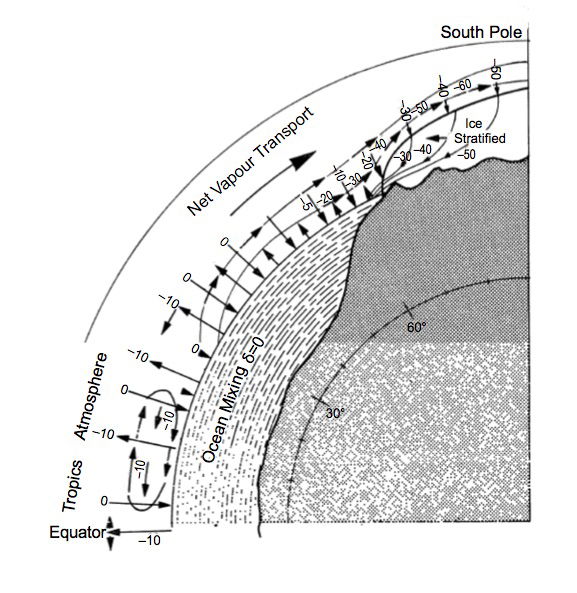
Fig. 2. Schematic of δ18O cycle of water vapour from the ocean to the Antarctic ice sheet. Figures in the ocean and atmosphere are δ18O values in ‰ (parts per thousand relative to SMOW). From Robin (1977), Fig. 7.
Since H218O is depleted in ice, the greater the global volume of ice, the greater the inventory of H218O residing in the oceans and atmosphere. Thus when there are significant ice sheets on the earth (as in the Pleistocene or as in Antarctica and Greenland today), the δ18O value in seawater and hence in marine fossils becomes a proxy for total ice volume: high values of δ18O in the oceans imply large ice volumes. This effect was first established by Shackleton (1967) and then further developed by Hays, Imbrie, and Shackleton (1976), who linked the Croll-Milankovitch astronomical theory of Pleistocene glacial intervals (“ice ages”) to the fluctuations in δ18O values found in ocean floor sediments. The astronomical theory proposes that variations in the earth’s orbital parameters, specifically eccentricity, obliquity (axial tilt) and axial precession, lead to variations in incoming solar radiation in summer at high latitudes (usually 65°N); glacial intervals are supposedly triggered when this radiation becomes too weak (Hays, Imbrie, and Shackleton 1976; Zachos et al. 2001); hence the title of the well-known and much-cited Hays, Imbrie, and Shackleton (1976) paper, viz. “Variations in the Earth’s Orbit: Pacemaker of the Ice Ages.”
Because of the apparent explanatory success of the astronomical theory, it now serves as a ruling paradigm in climate research and is often used to calibrate climate data chronologically, notably isotope records in deep-sea cores. However, this theory suffers from serious methodological flaws, described in detail by Oard (2005, 2007) and by Hebert (2016a, 2016b, 2016c). In summary, assuming the uniformitarian chronology, the most critical problems are: (1) orbitally-induced changes in solar radiation are very weak, especially the 100ka eccentricity cycle which appears, within the “astronomical forcing” paradigm, to have dominated climate variations over the last 400ka; (2) ice age cycles are in phase between Northern and Southern hemispheres, whereas the astronomical theory predicts the opposite—when the Northern hemisphere cools, the Southern should warm up, and vice versa; (3) causality, i.e. the warming which terminates a glacial interval sometimes precedes by several thousand years the change in solar radiation supposedly causing it; (4) the assumed age of 700ka for the Brunhes-Matuyama (B-M) magnetic reversal boundary, used in constructing age models for the analysis of Hays, Imbrie, and Shackleton (1976), has since been revised significantly upward to 780 ka (Hebert 2016c); (5) Hays, Imbrie, and Shackleton (1976) based their climate reconstructions on data from planktonic rather than benthic foraminifera. Since the former are much more likely to be affected by local short-term temperature variations (Hebert 2016a), how could Hays and co-authors be sure that their measured δ18O values represent a globally synchronous signal? Oard (2007) claims that the uniformitarian paradigm in this field continues as a “reinforcement syndrome,” and Hebert (2016a) concludes that the data sets have “evolved” over time, thus calling into question their supposedly objective nature.
When significant ice sheets exist on earth, other climate indicators are needed to quantify separately the contributions of temperature and ice volume to δ18O values, notably paleontological and geological evidence of lower sea levels and of the existence and extent of ice sheets (e.g. Clark et al. 2009; Francis 1988; Hambrey, Ehrmann, and Larsen 1991; Zachos et al. 2001). In a Flood scenario rapid changes in ocean conditions are expected, which may invalidate some conclusions based on the usual uniformitarian assumption of temporal near-equilibrium of oceanic δ18O levels; detailed consideration of this issue is beyond the scope of this article.
As anticipated by Urey et al. (1951), several factors complicate the use of fossil δ18O as a proxy for seawater temperature. These are summarized by Grossman (2012) as: disequilibrium precipitation of biogenic carbonate; the constancy of seawater δ18O; ecological influences; spatial variability versus temporal trends; and the preservation of the record through geological time. Here the major sources of uncertainty and complexity will be considered under the headings of (1) preservation of the original fossil δ18O; (2) “vital” or biological effects; and (3) environmental effects, notably seawater 18O levels. There is necessarily some interaction between environmental and vital influences because marine organisms usually respond in some way to changes in their environment (e.g. Hahn et al. 2012).
Preservation
The issue is whether oxygen isotope ratios in the fossil shell material are maintained intact or modified by the higher temperatures and pressures of burial during diagenesis or by subsequent chemical reactions. Oard (2003) cites analysis by Schrag (1999) of oxygen isotope records of planktonic foraminifera apparently indicating that Late Eocene and Oligocene tropical sea surface temperatures were up to 8°C lower than today’s, yet this part of geological history was supposedly characterized by a generally warm climate. Schrag’s solution was to invoke alteration by diagenetic recrystallization, which involves incorporation of relatively 18O-rich bottom water into the shells. As electron microscopy has shown, calcite can be added inside the shell or even replace its original structure, both effects being undetectable by standard microscopy (Oard 2003). Pearson et al. (2001) analyzed planktonic foraminifer shells from impermeable, clay-rich Late Cretaceous to Eocene deposits in Tanzania. Their samples were examined by electron microscopy to ensure that they were “exceptionally well preserved.” The inferred sea surface temperatures were 28–32°C, considerably higher than the figures given in most comparable previous studies. This further implies that recrystallization could have introduced major errors in previous studies, especially for planktonic foraminifera; fossils of benthic organisms such as brachiopods, bivalve molluscs, and benthic foraminifera are less prone to recrystallization because bottom water is consistently cold (typically ~2°C). Poor preservation of shell material may be indicated by opaque rather than translucent shell material as noted by Grossman (2012) for brachiopods and by Wycech, Kelly, and Marcott (2016) for planktonic foraminifera. Grossman (2012) emphasizes the need for extremely careful sample screening against chemical alteration before undertaking oxygen isotope paleothermometry and describes very detailed screening protocols.
Pérez-Huerta, Coronado, and Hegna (2018) systematically review the role of biomineralization in our understanding of the fossil record. They first note that biominerals consist of a mineral phase and a multicomponent organic matrix in varying proportions, although fossils often retain little or none of the organic phase. They then systematically describe: (1) the basic characteristics of biominerals. Although there is an immense variety of these in existence, they share a number of key recognizable characteristics, viz. hierarchical organization, biocomposite nature, unique mineralization mechanisms, biological crystallographic control, and common nanostructure organization (Pérez-Huerta, Coronado, and Hegna 2018, section 2); (2) how to recognize primary (unaltered) biominerals in fossils. Preservation of the original mineralogy depends mainly on whether it has crossed its solubility threshold, i.e. whether it has suffered dissolution because of unfavorable pressures, temperatures, or water chemistry arising during its diagenetic history. Thus for calcium carbonate fossils the original mineral form, e.g. aragonite or calcite, is important because aragonite is more soluble than low-Mg calcite; (3) the factors involved in diagenetic alteration of fossils and the techniques available for evaluating such alteration.
High-resolution modern techniques including scanning electron microscopy, energy-dispersive spectroscopy, cathodoluminescence microscopy, electron backscatter diffraction and Raman spectroscopy are now used to characterize the primary mineralogy of fossils and to detect and evaluate the effects of diagenetic alteration. These have recently been supplemented by atomic force microscopy (AFM) and field emission secondary electron microscopy (FEG-SEM) which can show biomineral structures down to nanoscale. A good example of the use of such techniques is the discovery by Balthasar et al. (2011) of relic aragonite in brachiopod shells from Ordovician and Silurian rocks; detailed characterization of the shell mineralogy was key to this discovery. However an important corollary is that in earlier studies of environmental indicators in fossils, undertaken before these highly sophisticated techniques became available, the exact state of preservation of the fossils was unknown, implying that the reliability of the results, e.g. temperature reconstructions from δ18O measurements, is uncertain.
Vital Effects
Marine organisms which produce fossils of interest for temperature reconstructions generally live at the same temperature as the ambient water (Urey et al. 1951). However biomineralization, the formation of their hard parts, is biologically controlled and therefore does not necessarily occur in isotopic equilibrium with seawater. Hence δ18O values in biominerals may not be truly representative of ambient conditions.
Examples of identifiable vital effects in planktonic foraminifera were reported by Bemis et al. (1998) in laboratory culture experiments on the symbiotic species Orbulina universa and the non-symbiotic Globigerina bulloides; the temperature range was 15–25ºC. O. universa, which lives in the photic zone, hosts photosynthetic algal symbionts which are thought to modify the carbonate ion [CO32-] concentration and hence pH locally depending on the light level (Pearson 2012). This in turn modifies the δ18O difference between the shell calcite and the seawater (δ18Osc–δ18Osw) such that in high light (~16 times stronger than low light1 and with normal ambient CO32- levels, δ18Osc is depleted on average by 0.33‰ relative to its low-light value. This change corresponds to temperatures overestimated by ~1.5ºC, possibly explaining a widely observed discrepancy of this magnitude between temperatures based on standard T/δ18O calibrations and temperatures measured in-situ for planktonic and shallow water benthic foraminifera (Pearson 2012). In the chambered non-symbiotic G. bulloides, the main vital effect is ontogeny, which means that during shell growth successive chambers are progressively enriched in 18O relative to earlier ones; this introduces a shell-size effect into temperature–(δ18Osc–δ18Osw) calibrations. Thus for example the slope of the T/δ18O curve for an 11-chambered shell is –5.07(±0.22), and for a 13-chambered shell –4.77(±0.27).
Fontanier et al. (2006) studied microhabitat and seasonal effects on the stable oxygen and carbon isotopes in seven species of benthic foraminifera. They found that while Uvigerina peregrina forms its test in close equilibrium with bottom water δ18O, all the other species (including U. mediterranea, a sister species within the same genus) maintain different but practically constant offsets against calcite formed in equilibrium with bottom water δ18O. They found no systematic relationship between the foraminiferal habitat depth within the bottom sediment and the foraminiferal δ18O offset against calcite in equilibrium with bottom water (designated Δδ18O≡δ18Osc–δ18Oec). Basak et al. (2009) undertook a similar isotopic study of five species of live benthic foraminifera. They found little interspecific variation in Δδ18O values, and no systematic variation with habitat depth, which they understood to imply that metabolic rate, which depends on nutrient supply and oxygen level, does not influence 18O fractionation in these organisms.
Ishimura et al. (2012) investigated the isotope characteristics of multiple species of benthic foraminifera and found not only interspecific variations in Δδ18O values but also intraspecific variations (i.e. between individuals of the same species). In all species investigated they found an ontogenetic effect: 18O enrichment in the shell calcite increased with specimen weight, the largest specimens having δ18Osc values closest to equilibrium calcite. Ishimura et al. (2012) concluded that (1) the species showing least intraspecific variation in Δδ18O are the most suitable for temperature reconstructions, their best candidate being Bulimina aculeata, and (2) carbonate ion [CO32-] concentration may be a major contributory factor to the Δδ18O variations seen in the most variable species. Bhaumik et al. (2017) investigated microhabitat-related isotope variations between pairs of benthic foraminiferal species with overlapping ranges of habitat depth and found that only Bulimina marginata showed δ18O enrichment with increasing habitat depth, interpreted as due to lower carbonate ion concentrations and hence reduced pH. Other possible vital effects noted but not directly investigated by Bhaumik et al. (2017) include respiration and “kinetic effect”; the latter, or kinetic fractionation, occurs in unidirectional (non-equilibrium) reactions and enhances the resulting degree of fractionation. A good example is photosynthesis, in which plants preferentially absorb 12C from atmospheric CO2 and therefore become depleted in 13C relative to inorganic carbon.
In order to construct a consistent isotope record, isotope fractionation effects and different life styles of the organisms must be calibrated to a common standard. The most useful organisms for this purpose are brachiopods, which are represented by fossils throughout the Phanerozoic and are distributed across practically all benthic marine environments (Bitner and Cohen 2013; Wright 2014). Hence Prokoph, Shields, and Veizer (2008) introduce an “articulate brachiopod standard” (ABS), noting that: (1) the articulate brachiopod group has a stratigraphic range from the Cambrian to the present; (2) brachiopod habitats and their vital effects have been studied; (3) the diagenetic alteration of the shells can be evaluated; (4) brachiopod isotope data are available for almost the entire Phanerozoic; and (5) their primary shell material consists of low-Mg calcite for which a transfer function to water temperature can in most cases be established.
The question of how vital effects influence proxy measurements is reviewed for bivalve molluscs, cephalopods and brachiopods by Immenhauser et al. (2016), who consider traditional proxies including carbonate δ18O, δ13C, Mg/Ca, and Sr/Ca values, and more novel proxies including carbonate clumped isotopes (designated Δ47, discussed in Part 2 of this series). Immenhauser et al. (2016) conclude with regard to δ18O data from molluscs and brachiopods (p.29) that:
Under constant temperature and a non-stressed environment most molluscs and brachiopods fractionate oxygen isotopes near equilibrium with the ambient aquatic medium, at least with reference to some portions of their exoskeletons or endoskeletons and when corrected for relevant parameters.
However Immenhauser et al. (2016) also state that unanswered questions remain as to the impact of organic matrices and metastable precursor carbonate on oxygen isotope fractionation. They note that, although brachiopods generally secrete their primary (inner) calcite fibers close to oxygen isotopic equilibrium with the seawater, some studies have reported kinetic and metabolic isotope fractionation differing between taxa and even within a single brachiopod valve, and that from the bulk isotopic range across the secondary shells of two congeneric brachiopod species seawater temperatures were overestimated by 24ºC. Much of this kind of variation is now thought to be due to a “MgCO3 effect” (Brand et al. 2013); incorporating MgCO3 into brachiopod shell calcite affects its δ18O level and hence the T/δ18O calibration equation. Having investigated this effect in several species of modern brachiopods from a range of globally-distributed sites, Brand et al. (2013) proposed a new calibration equation for articulated brachiopods:
where δ18Osc and δ18Osw are the shell calcite and seawater δ18O levels respectively and δMg is an adjustment in δ18O of +0.17‰ per mol% MgCO3 incorporated into the shell calcite. Although δ18Osc and δMg can in general be measured for a single fossil shell, use of equation (2) presupposes that δ18Osw is either known or can be assumed from additional information. Brand et al. (2013) suggest that similar adjustments for the MgCO3 content of calcite in inarticulated brachiopods and other high-Mg calcitic marine invertebrates would enable their use as valuable paleotemperature archives.
It is perhaps worth noting here that while biomineralization, specifically the formation of calcitic shells by marine invertebrates, is biologically controlled it is also affected by seawater chemistry (Pérez-Huerta, Coronado, and Hegna 2018). Thus for example calcitic bivalve molluscs grown in artificially high-Mg seawater were found to secrete aragonite on their interior shell surfaces (Checa et al. 2007). Variations in Mg/Ca in the oceans through the Phanerozoic and its effects will be discussed in Part 2 of this series.
Seawater 18O levels
The 18O level in fossil shell material depends on both its formation temperature and the δ18O value of the seawater: we assume either that the global ice volume is negligible or that its effect on seawater δ18O values has already been accounted for. There is naturally some spatial variation in the 18O level in the oceans. Thus according to Grossman (2012), the bulk of modern seawater, represented by deep water masses, has a relatively narrow δ18O range from about –0.6‰ (Antarctic Bottom Water) to +0.1‰ (North Atlantic Deep Water). Open-ocean surface waters are more variable, ranging from about –0.5‰ in the Southern Ocean to +1.4‰ in the dry subtropical zone in the North Atlantic. 18O variability in the surface waters of enclosed seas, such as the Arctic Ocean, Mediterranean Sea, and Red Sea, is even larger, roughly –2‰ to +2‰, owing to the varying balance of evaporation and precipitation. There is an acknowledged correction for the effects of latitudinal variation in the precipitation-evaporation balance in the Southern Hemisphere (Grossman 2012). Close to continents, mixing with fresh water can lower δ18O by an amount depending on the δ18O of the river water, which contributes to the correlation between salinity and seawater δ18O (LeGrande and Schmidt 2006; Polyak, Stanovoy, and Lubinski 2003); in some circumstances this correlation means that δ18O becomes primarily a proxy for water density rather than temperature (Lynch-Stieglitz, Curry, and Slowey 1999). Other factors noted by Grossman (2012) include water depth, global ice volume, which affects salinity because freezing seawater excludes salt, and precipitation, which reduces seawater δ18O values locally (LeGrande and Schmidt 2006).
Spatial variability of δ18O in Holocene oceans is thus reasonably well understood. However temporal variability has been controversial and harder to pin down. Practically all investigators, notwithstanding scatter and variations in both directions, have found that fossil 18O levels increase progressively upwards through the geological record. Some have treated this as a diagenetic artifact (e.g. Killingley 1983), while others have deduced a rising level of 18O in the oceans, and yet others have inferred long-term cooling. Veizer and Prokoph (2015) argue that the oceanic 18O level has risen progressively through geological time, citing: (1) the across-the-board consistency of the secular trend in 18O measurements, including those where sample integrity was carefully checked, and (2) the corresponding secular trend, confirmed independently by different groups, in other isotopic and element ratios. These include carbon, sulfur, calcium, radiogenic and stable strontium isotope ratios, and Sr/Ca ratios (Prokoph, Shields, and Veizer 2008). Veizer and Prokoph (2015, 93) state:
It is therefore inconceivable to argue that the atoms of oxygen, the dominant structural unit of calcite crystals, must have been massively exchanged during diagenesis while at the same time none of the other major and trace elements or isotopes were affected.
Hence Veizer and Prokoph conclude that the secular trend in fossil δ18O values indicates increasing oceanic 18O levels rather than changing temperatures. This must have involved oxygen exchange between the water and hot silicate rocks, for example at mid-ocean spreading ridges. Interaction with rocks at temperatures above 350°C causes 18O enrichment of seawater; conversely 18O depletion occurs at lower temperatures (Walker and Lohmann 1989). Changes in seawater chemistry revealed in coupled variations in the mineralogies of marine aragonite limestones and potash evaporites through the Phanerozoic have been attributed to variations in the mid-ocean ridge hydrothermal brine flux, due in turn to variations in the rate of ocean crust production (Hardie 1996; Stanley, Ries, and Hardie 2002). Thus seawater chemistry, defined in terms of ion content (e.g. Mg/Ca and Sr/Ca) and isotope ratios (e.g. δ18O), has undoubtedly changed significantly over geological time because of crustal movements and changes in heat and mass transfer at the ocean floor. The challenge is to integrate the changes apparent in the geological record into a Flood-based geological paradigm.
2. Appraisal of Oxygen Isotope Data
For Flood models such as CPT (Austin et al.1994), the Cenozoic represents the post-Flood period, characterized in its late stages by the growth of ice sheets and an Ice Age (Oard 1990). As noted earlier, in other Flood models the correspondence of ocean floor development with Flood chronology will vary depending on where the Flood/post-Flood boundary is placed in the geological record; this question is considered further in section 3.
Cenozoic oxygen isotope data are reviewed by Zachos et al. (2001), based on δ18O measurements on the calcareous fossil remains of two types of common, long-lived benthic foraminifera, Cibicidoides and Nuttallides. Zachos et al. treat the δ18O record as a proxy for ocean floor temperature up to the late Eocene, when the Antarctic ice sheet began to form, around 35MaBP (before present) in the uniformitarian chronology. From the early Oligocene they treat δ18O as a qualitative indicator of ice volume. Although the trend is not monotonic, the overall change in δ18O is +5.4‰ over the whole Cenozoic, which they resolve into +3.1‰ to represent deep-sea cooling, +1.2‰ for growth of the Antarctic ice sheet and +1.1‰ for subsequent growth of Northern Hemisphere ice sheets. A more comprehensive δ18O data compilation is given by Cramer et al. (2009). The highest global ocean-floor temperatures in the Cenozoic inferred from δ18O data are approximately 12–13ºC (see fig. 3), occurring at the Paleocene-Eocene Thermal Maximum (PETM) at about 55 Ma and during the Early Eocene Climate Optimum (EECO) at about 51 Ma in the uniformitarian chronology (Cramer et al. 2009; Mudelsee et al. 2014; Zachos et al. 2001). This temperature limit can be taken as robust since it is based on low-Mg calcite fossils with minimal MgCO3 effect on their δ18O values (cf. equation 2), and the contribution of the secular trend in seawater 18O levels identified by Veizer and Prokoph (2015) is insignificant for the Cenozoic.
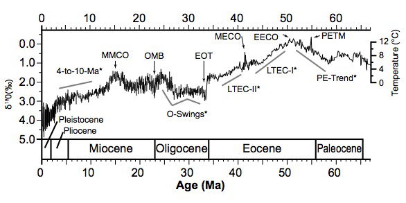
Fig. 3. Global Cenozoic δ18Ovalues from benthic foraminiferal shells found in marine sediment cores. The temperature scale, which assumes an ice-free ocean, employs the transfer function used by Zachos et al. (2001). Since ice sheets appeared around the Eocene-Oligocene transition, indicated temperatures thereafter are too low, rising δ18O values indicating growing ice volume as well as low temperatures. From Mudelsee et al. (2014), Fig. 1.
The review of δ18O data covering most of the Phanerozoic up to the present (i.e. from 512Ma in the uniformitarian chronology) by Veizer and Prokoph (2015) includes the data published by Zachos et al. (2001) and Cramer et al. (2009), together with data from several other sources. Altogether, measurements from over 58,000 low-Mg calcite fossil marine shells are included. The Paleozoic portion of the record is covered almost entirely by brachiopods while other taxa dominate the Mesozoic and Cenozoic. Fig. 4 [taken from Fig. 1 in Veizer and Prokoph (2015)] shows, despite distinct fluctuations, a secular trend of +6±1‰ over the whole dataset. Shells secreted at low temperatures are extremely scarce; almost none from the Paleozoic plot above the 0‰ level of δ18O for modern calcite.
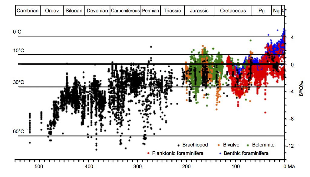
Fig. 4. G δ18O of Phanerozoic low-Mg fossils (57,146 data points), taken from Fig. 1 in Veizer and Prokoph (2015). Temperature estimates are based on the Visser, Thunell, and Stott (2003) transfer function, assuming the present day δ18O value of 0‰ SMOW for seawater. Veizer and Prokoph (2015) give details of all the data and their sources.
If the observed secular trend is interpreted through a single δ18O/ocean temperature calibration with present-day SMOW (Standard Mean Ocean Water) as the 0‰ reference, it implies considerable cooling from 50–55°C in the mid-Cambrian to a present-day average of 15°C; ocean temperatures today lie between about 0°C and a sharply-defined maximum of 30–32°C on the surface (NOAA 2018). As noted previously, Veizer and Prokoph argue rather that the δ18O trend is due to a secular increase in the 18O level in ocean water since the Cambrian.
Oxygen-18 levels in Precambrian strata show a similar trend (Jaffrés, Shields, and Wallmann 2007; Prokoph, Shields, and Veizer 2008; Shields and Veizer 2002; Veizer and Hoefs 1976), though in uniformitarian terms the change is slower than in the Phanerozoic. Thus Precambrian δ18O values are lower than Phanerozoic values. Some early papers inferred very high Precambrian water temperatures. For example, Knauth and Epstein (1976) deduced from δ18O values in Archean cherts that water temperatures were up to 70°C at 3Ga (billion years) ago, but others have questioned the accuracy of this parameter as a temperature proxy. Thus Walker (1982) contends that, since evaporitic gypsum cannot form above 58°C yet is found in Precambrian strata, the water temperature could not have been above 58°C. Walker also sees the continued presence of life in the Precambrian as implying temperatures not exceeding 60°C. In contrast, Knauth and Lowe (2003) and Knauth (2005) argue from δ18O measurements of cherts from the Swaziland Supergroup that Archean temperatures lay in the range 55–85°C. Further studies suggest Archean ocean temperatures much closer to present-day values. Thus from analysis of both oxygen and hydrogen isotope ratios in an Archean chert, Hren, Tice, and Chamberlain (2009) deduce ocean temperatures not exceeding 40°C, while temperatures derived from oxygen isotope measurements in Archean phosphates lie in the range 26–35°C (Blake, Chang, and Lepland 2010), roughly equivalent to present-day values. A recent study of volcanic rocks and cherts from the Barberton Greenstone Belt in South Africa (De Wit and Furnes 2016) reveals the existence of deep-water hydrothermal systems in a relatively cold Archean environment; temperatures inferred from δ18O data range from 30°C to above 200°C. Could part of the reason for apparently conflicting temperature indications from studies of Archean rocks be an extremely heterogeneous formation environment in terms of temperature and water chemistry?
3. Interpretation of the Data in Terms of Flood Geology
All discussions of complicating issues in the secular literature presuppose the uniformitarian chronology, within which the assumption of a climate system approximating to steady state is a meaningful concept. Inarticulated brachiopods typically live for ~1–10 years and articulated brachiopods for ~3–30 years (Bitner and Cohen 2013; Emig 1997; Immenhauser et al. 2016), while bivalves can live for 50 years or more and deep-water species up to 100 years (Jones 1989). These life spans are short compared with climate change time scales typically contemplated within uniformitarian geology; in that framework the concept of quasi-steady state may be appropriate.
However, within a biblical timescale, in which (say) most of the Phanerozoic represents deposits laid down during the Flood year, conditions must have changed rapidly. Thus in a CPT Flood scenario, there will probably have been rapid, large-scale exposure of hot mantle rock to ocean water, resulting in considerable exchange of oxygen and significant change in the oceanic 18O level. Furthermore the breaking up of “the fountains of the great deep” (Genesis 7:11), perhaps as a result of the dewatering of rising, depressurizing magma, could have injected into the oceans a large quantity of water with a different δ18O value from that of the pre-Flood ocean. Unless it has suffered recrystallization, the calcite in fossil shells deposited during the Flood year, many of which represent animals killed and buried in the Flood, must represent ambient conditions immediately before or in the early stages of the Flood. If 18O levels changed significantly during the Flood (though the direction and magnitude of change cannot be predicted), this change should be reflected in the calcite in post-Flood fossil shells. In the standard CPT Flood model (Austin et al. 1994) these would be the lowest-level Cenozoic fossils, i.e. from the Paleogene; in Flood models which place the Flood/post-Flood boundary higher in the stratigraphic record these fossils would be found correspondingly higher. Inspection of fig. 3 suggests no obvious major change in the δ18O level either at the K-Pg interface or above it except possibly at the PETM or EECO.
Some who accept CPT as the basic explanatory framework for the Flood would now place the Flood/post-Flood boundary somewhere between the K-Pg boundary and the Pliocene/Pleistocene boundary. Thus Baumgardner, who developed a coherent physical model for the mechanism underlying CPT (Baumgardner 1986, 1994a, 1994b, 2003) and was a co-author of the Austin et al. (1994) paper, places the Flood/post-Flood boundary in the Pliocene (Baumgardner 2005, 2012). Snelling (2009) argues that this boundary must lie somewhat above the K-Pg interface on account of the large amount of geological work in evidence in rocks above the Cretaceous. Clarey (2016) firmly supports the CPT model but does not say exactly where he would place the Flood/post-Flood boundary, while Ross (2012), who also subscribes to CPT, inclines to the standard CPT placement of this boundary.
Not all Flood models view the geological record in this way. Brand (2007) assumes considerable geological activity both before and after the Flood, though he sees the Flood as the single most significant event in earth history. His model does not predict a clear end-of-Flood marker in the geological record. Gentet (2000), in his CCC (Creation/Curse/ Catastrophe) model, acknowledges the order of the stratigraphic column as real and treats the different fossil assemblages in the geological record as representing different ecological zones rather than geological periods. Consequently, although Gentet believes that Precambrian rocks date from Creation Week, he places the pre-Flood/Flood and the Flood/post-Flood boundaries in different strata within the geological column in different locations; however most creation scientists view the column as lithostratigraphically and biostratigraphically real whilst maintaining caution about the details (Snelling et al. 1996; Tyler and Coffin 2006). Oard (2016), who has written extensively on Flood-related issues but who does not accept CPT, adopts the “Late Cenozoic Boundary Model,” which places the Flood/post-Flood boundary at different stratigraphic levels in different locations, but all corresponding to a “Late Cenozoic” designation. None of these alternatives provides a coherent physical mechanism to explain the Flood in the same way as CPT, nor is it possible to make any meaningful comparison between model predictions and data for seawater temperatures through the Flood/post-Flood boundary except where a clear end-of-Flood marker has been defined.
If the geological record is understood in terms of a Recolonization model, in which Flood deposits correspond largely to Hadean and Archean rocks (Tyler 2006), practically all accessible fossil marine shells will have been deposited over the subsequent 4400 or so years. Since these shells would not then have been deposited during the Flood, steady-state conditions might be a better approximation to reality. However, Tyler envisages that the recovery and recolonization of the earth after the violence of the Mabbul would have been punctuated by further catastrophic events, implying that for much of geological history one cannot necessarily assume steady state. Given the stratigraphically poorly defined end to the Flood in this model, end-of-Flood seawater temperature predictions for this model cannot be compared with geological data, although Tyler (2006) suggests that the high Archean water temperatures indicated by the data of Knauth and Lowe (2003) and Knauth (2005) would be consistent with hot ocean water at the end of the Flood.
A number of creation scientists (e.g. Austin et al. 1994; Vardiman 2013) have taken at face value published paleotemperatures based on δ18O data, apparently without considering the validity of the δ18O/temperature calibration used in their sources. However Vardiman (1996b) outlines the basics of oxygen isotope thermometry and discusses many of its complicating factors. He cites: (1) biological factors (e.g. disequilibrium effects in foraminifera); (2) diagenetic effects (e.g. recrystallization, biasing of a fossil assemblage due to preferential solution of the “warmer” fraction); (3) ecological factors (e.g. seasonal migration), which must be accounted for in linking inferred temperatures with climate; (4) in a Pleistocene context, foram habitat changes between glacial and interglacial conditions. Vardiman (1996b) also acknowledges the impact of the seawater δ18O value on temperature estimates, but only in relation to the growth and retreat of Pleistocene ice sheets. Vardiman does not mention the effect on 18O levels of interactions between hot mantle rocks and seawater, nor does he consider the possibility of a long-term trend in global oceanic 18O levels. He concludes that in a Flood model context the accuracy of past temperature estimates is unlikely to be better than 3 or 4°C.
Regardless of the particular Flood scenario assumed, creation scientists must inevitably interpret the 18O record in marine fossils differently from uniformitarian scientists, mainly because their timescales are much shorter. Furthermore creation scientists have not thus far considered the possibility (discussed above) of a long-term increase in ambient 18O levels. Thus further investigation is needed to clarify our interpretations of δ18O values in pre-Cenozoic marine fossils and their implications for past ocean temperatures.
Surface Heat Flows
1. General Picture
The earth is steadily losing internal heat. According to Pollack, Hurter, and Johnson (1993), the total outward surface heat flow is 44.2×10¹²W, or 44.2TW, which implies an average heat flux of 87mWm-2. Davies and Davies (2010) estimate a figure of (47±2)TW for the total outward heat flow; the uncertainty of ±2TW is their 2σ statistical uncertainty. The division between continents and oceans given by Davies and Davies is shown in Table 1.
| Area(km2) | Heat Flow(TW) | Mean Heat Flux(mWm-2) | |
|---|---|---|---|
| Continent | 2.073×1080 | 14.70 | 70.90 |
| Ocean | 3.028×1080 | 31.90 | 105.40 |
| Global Total | 5.101×1080 | 46.70 | 91.60 |
The major contributions to the total surface heat flow are radiogenic heat production in the crust and mantle, heat flow from the core, and secular cooling of the mantle (Furlong and Chapman 2013). These authors estimate that approximately half the earth’s total heat budget is due to heat released from the core through the CMB and to radiogenic heat generated in the lower mantle. Partitioning of the remainder (20–25TW) between radiogenic heat production (largely in the continental crust) and secular cooling of the mantle is the subject of debate among uniformitarian scientists.
According to Furlong and Chapman (2013), continental heat flow largely arises from radiogenic heat production in the lithosphere (notably the continental crust), while oceanic heat flow is dominated by lithospheric cooling away from mid-ocean ridges (MORs). Fig. 5 (their Figure 1) schematically illustrates the partitioning of surface heat flows. The temperature field in the oceanic lithosphere is well constrained, the surface heat flux declining with distance from the MOR. In contrast, the continental temperature field is complex and generally poorly resolved because vertical heat generation profiles are not well known, there is considerable lateral variation in heat production and continental rocks have undergone a complex tectonic history.
Below the plate boundary corresponding to a mid-ocean ridge heat is transported upwards by upwelling hot mantle material participating in mantle convection. As this material rises and phase changes due to decompression take place, the axial heat flux consists of (1) the release of latent heat of crystallization of basaltic magma, and (2) the heat lost by cooling of magma down to hydrothermal temperatures ~350ºC (Elderfield and Schultz 1996). The resulting rock accretes to the base of the spreading plates, leading to plate thickening with distance from the MOR. According to Turcotte and Schubert (2002, section 4.16) the lower boundary of the plate may conveniently be defined by the 1600K isotherm, which corresponds to the temperature below which mantle rocks do not readily deform on conventional geological timescales; however the exact choice of isotherm temperature is not critical for subsequent analysis. Turcotte and Schubert (2002, section 4.16) ignore hydrothermal effects and undertake a formal heat conduction analysis which gives a plate thickness of ~2(κt)½, where κ is the thermal diffusivity of the plate material (taken to be 10-6m2s-1) and t is the time since moving away from the MOR. Fig. 5 qualitatively depicts the plate thickening process.
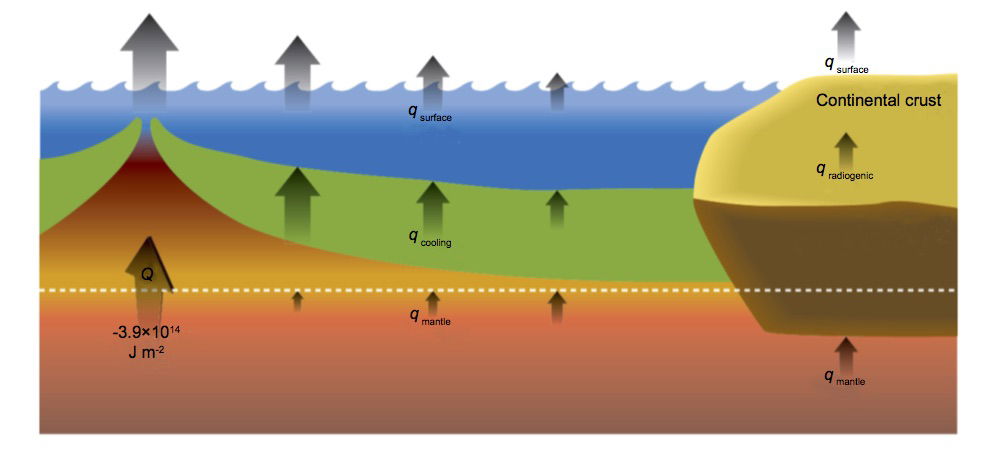
Fig. 5.Schematic of heat flow partitioning at various levels in both oceanic and continental lithosphere. From Furlong and Chapman (2013), Fig. 1
However Furlong and Chapman (2013) view the rheologically plate-like behavior of oceanic lithosphere as resulting from its compositional properties, viz. water content, rather than simply from its thermal properties, and suggest that this has important consequences for the transfer of heat from the deeper mantle into the lithosphere. They first note that mantle material is emplaced at shallow levels as a result of partial melting and separates into crustal and residual mantle components (see fig. 5). Furlong and Chapman cite the work of Hirth and Kohlstedt (1996) who reevaluated high-pressure experimental data on the viscosity of olivine aggregates (dunite) in relation to water content, arguing that olivine is the rheologically dominant component of peridotites. Hirth and Kohlstedt conclude that there is an excess of water in the MOR basalt (MORB) source region, corresponding to a pressure of 300MPa, which implies that the viscosity there is hundreds of times lower than in dry olivine aggregates. Hirth and Kohlstedt thus estimate that the partial melting which generates new oceanic crust starts ~115km down and dehydrates the associated mantle, leading to a mechanical layering of dry mantle above the 60–70km depth interval with wet mantle beneath. Consequently viscosity decreases by 2–3 orders of magnitude from above to below depths of approximately 70–100km. Hirth and Kohlstedt (1996, Abstract) conclude:
These observations indicate that the base of an oceanic plate is defined by a compositional rather than thermal boundary layer, or at least that the location of the thermal boundary layer is strongly influenced by a compositional boundary, and that the evolution of the oceanic upper mantle is strongly influenced by a viscosity structure that is controlled by the extraction of water from olivine at mid-ocean ridges.
Furlong and Chapman (2013) deduce that there is little upward conductive heat flow at 100km depth; the conductive heat flux at the base of the plate increases to no more than about 17mWm-2 as the plate material cools and moves away from the MOR; for comparison, the average surface oceanic heat flux is 105.4mWm-2 (see Table 2), a typical minimum is 48mWm-2 (Stein and Stein 1992), and the maximum in MORs is of order 450mWm-2 (Davies and Davies 2010). Thus since very little radiogenic heat is produced within the oceanic lithosphere (≈4mWm-2, Parsons and Sclater 1977), most heat emerging from young ocean regions must result from secular cooling. As indicated in fig. 5, the surface heat flux decreases with distance from the MOR, and the basal heat flux from the mantle below 100km, although small, becomes a progressively larger fraction of the total (Furlong and Chapman 2013). Furlong and Chapman estimate that a total of ~3.9×10¹⁴ Joules (per square meter of surface area of fresh oceanic lithosphere) is deposited in the upper 100km of the region, an enormous heat load if we are considering biblically-compatible timescales.
| Isotope | Energy/Atom(MeV) | μW/kg of Isotope | μW/kg of Element | Estimated total earth content (kg) | Total heat (TW) | Total heat 4.5 Ga ago (TW) |
|---|---|---|---|---|---|---|
| 238U | 47.70 | 95.00 | 94.350 | 12.86×10160 | 12.210 | 24.50 |
| 235U | 43.90 | 562.00 | 4.050 | 0.0940×10160 | 0.530 | 44.40 |
| 232Th | 40.50 | 26.60 | 26.60 | 47.9×10160 | 12.740 | 15.90 |
| 40K | 0.710 | 30.00 | 0.00350 | 7.77×10200 | 2.720 | 33.00 |
| Totals0 | 28.20 | 117.80 |
Stacey and Davis (2008), writing in uniformitarian terms, consider both ocean depth and ocean floor heat flux as functions of age, using the data and models of Stein and Stein (1992) and Stein (1995). The first cooling model used by these authors is a simple half-space model, with heat loss at the ocean floor both by conduction and by hydrothermal circulation of seawater. As the oceanic lithosphere cools, it contracts, its density increases, and its upper surface subsides. Consequently ocean depth increases, an effect enhanced by the increased water loading. However, model plots based on this analysis do not fully reproduce the data; after 30Ma the heat flux remains roughly constant, and after 70Ma the ocean depth levels out. A preferred alternative known as the plate model assumes that mature lithosphere reaches a limiting thickness, after which it ceases to cool further and behaves like a plate in steady state, its lower boundary maintained at a fixed temperature by contact with the asthenosphere (Richardson et al. 1995; Stein and Stein 1992). Another alternative assumes that the lower boundary of the oceanic lithosphere is at a fixed temperature (i.e. it coincides with an isotherm) and is subject to a constant upward convective heat flux; this is known as the CHABLIS (Constant Heat flow Assigned on the Bottom Lithospheric ISotherm) model (Crough 1975; Doin and Fleitout 1996). Both plate and CHABLIS models produce good fits to surface heat flux data for old lithosphere, but CHABLIS predicts continuing subsidence well beyond 80Ma, and the proportion of global mantle cooling due to erosion of material from the base of the lithosphere by secondary convection is 40% (the remaining 60% is due to subduction), much higher than in the plate model (Doin and Fleitout 1996). Although both models predict a lithospheric thickness (defined by a particular isotherm) of about 80km after 100Ma, the CHABLIS lithosphere continues to thicken well beyond this point. Another widely-observed feature of oceanic heat flows is that all conduction-based models significantly overpredict surface heat fluxes for relatively young oceanic lithosphere; this is attributed to ventilated hydrothermal circulation recharge and discharge at crustal outcrops or areas of thin sediment cover (Hasterok, Chapman, and Davis 2011).
In the plate model the asthenosphere, unless it is continuously and rapidly replaced, can only supply the heat flow needed to keep the base of the lithosphere at a fixed temperature by cooling, which must lead to lithospheric thickening. Stacey and Davis (2008) note that: (1) there is indeed seismic evidence of continuing lithospheric thickening, and (2) although hydrothermal cooling of young ocean lithosphere is certainly observed and modifies the vertical temperature profile through the upper few kilometers, attempts to model it had not been fully successful. Since surface heat flux and ocean depth stabilize on different time scales, Stacey and Davis suggest that two additional effects need to be modeled. They raise two possibilities: (1) hydrothermal circulation extending deep into the lithosphere, redistributing heat but not necessarily exhausting it into the ocean; (2) an asthenosphere which thickens as it approaches a subduction zone. However they do not consider that a fully satisfactory solution is available.
Given that the earth’s ocean basins are geologically young, few areas being older than early Jurassic (Müller et al. 2008), and that most creation scientists regard Jurassic rocks as Flood deposits, these basins must have formed during and since the Flood, and most oceanic lithosphere must have cooled to its present state within that time, i.e. in no more than 4500 years, probably far less. As noted above, the heat load of ~3.9×10¹⁴Jm-2 of fresh ocean lithosphere due to material surfacing at MORs (Furlong and Chapman 2013) is enormous, more than 30 times enough to boil off the oceans if deposited very rapidly. The associated “heat problem” is to determine how the cooling was accomplished in a short time (Barnes 1980). A first attempt at this was made by Worraker and Ward (2018), who used the framework provided by the plate model of Stein and Stein (1992), suitably modified to accommodate biblically-compatible time scales, by invoking a transient subsurface heat sink. This was treated as a function of both space and time combined with rapid but decelerating plate motion. However, even with the optimum choice of model parameters available, Worraker and Ward were unable to find even a remotely satisfactory solution: predicted surface heat fluxes were far too high and ocean depth profiles far too sharp. These problems stem from the existence of a narrow near-surface thermal boundary layer, an inevitable consequence of the short time scales imposed in the model. Further details of this work and a discussion of possible ways forward in solving this heat problem, probably including hitherto neglected geophysical effects (e.g. deep hydrothermal convection, superheated steam jets, etc), will be given in Part 4 of this series.
2. A Creationist Resolution of Problematic Heat Flow Data
Baumgardner (2000) has shown that a longstanding puzzle for the earth science community, namely the widely-found correlation between surface heat flow and the measured radioactivity of surface continental igneous rocks, can be neatly explained within the creationist paradigm. Uniformitarian explanations appear rather contrived. For example, (1) Roy, Blackwell, and Birch (1968) invoke a vertical column of rock 7–11km deep through which the level of radioactivity is practically uniform and is closely correlated with the surface rock type, and (2) Lachenbruch (1970) suggests a model in which radiogenic heat production decreases exponentially with depth. Subsequent investigations in crystalline continental crust elsewhere (e.g. in Russia and in Germany) have also shown no variation of radiogenic heat production with depth—rather, it follows lithology (Clauser et al. 1997; Pribnow and Winter 1997). The problem is discussed by Furlong and Chapman (2013), who prefer Lachenbruch’s (1970) exponential model to the alternatives, but do not offer a definitive solution.
Baumgardner (2000) proposed a modest pulse of accelerated nuclear decay (AND) during the Genesis Flood (~5000 years ago) which produced an episode of increased radioactive heating whose aftermath now dominates the surface heat flow in the host plutonic rocks. This would have raised the temperature of the host rocks by an amount proportional to the concentration of heat-generating elements. Baumgardner estimates that today’s observed heat flows can be explained in terms of 190,000 years’ worth of accelerated decay through a depth of approximately 1km. The resulting temperature rise lies between 5.5K and 22K, corresponding to the approximate lower and upper limits respectively of present-day radiogenic heating in granites. These figures are perfectly credible and the depth requirement is more plausible than the uniformitarian assumption that the surface level of radioactivity is correlated downwards to depths of about 10km.
From his contributions to the RATE project, Snelling (2005a, 2005b, 2005c, and pers. comm.) concluded that:
... the RATE project demonstrated that there was physical evidence (fission tracks and radiohalos) for only 500–600 million years’ worth of accelerated radioactive decay only during the Flood.
Given that the Genesis Flood lasted about a year, Snelling’s comment implies an overall acceleration factor of about 6×10⁸, or 600 million, considerably larger than the value of 1.9×10⁵ implied by Baumgardner’s results. To reconcile this difference note that Baumgardner’s analysis deals only with the net additional heating of the rocks during the Flood as a result of AND; given a sufficiently strong additional cooling mechanism operating simultaneously during the Flood, there is no conflict. The challenge is to identify a cooling mechanism strong enough to limit the temperature rise in granite plutons to the ~20K level deduced by Baumgardner.
A rough idea of the magnitude of this problem may be obtained by considering the total radiogenic heat generated during the Flood year as a result of AND within typical granite, and comparing it with the heat needed to melt the granite. Taking the average present-day radiogenic heat production in granite as 1.05×10⁻⁹ Wkg-1 (Table 3), the total heat generated by 6×10⁸ years’ worth of radioactive decay is 1.99×10⁷ Jkg-1. Taking the granite melting point as its typical liquidus temperature of 1550K, its latent heat of melting as 4.2×10⁵Jkg-1 and its specific heat capacity as 830Jkg-1K-1 (Stacey and Davis 2008, Table A.6), and assuming a starting temperature of 300K (=27ºC), the heat needed to melt it is 1.46×10⁶ Jkg-1. The predominant mineral component of granite, silica (SiO2 ) has a boiling point at 1 bar of 3177K and an enthalpy of vaporization of approximately 1.2×10⁷Jkg-1 (Kraus et al. 2012). Thus if delivered adiabatically (i.e. in a time short compared with the thermal diffusion time scale of the granite body, which would be the case for anything larger than ~5m across) the AND heat load is more than 13 times enough to completely melt the granite, and may even be enough to vaporize it. Although this estimate is somewhat misleading (e.g. much granite was undoubtedly emplaced during rather than before the Flood, etc.), it suggests nevertheless that a powerful cooling mechanism operating at the same time as AND is needed. This issue is considered further in later articles in this series.
3. Inventory of Heat-Producing Radioactive Elements
Baumgardner (2000) reviews the distribution of radioactive isotopes in the earth from a creationary perspective. He notes that mainstream models of the earth’s chemical make-up are based mainly on data from present-day rocks, and are therefore generally robust and reliable. Notable features include: (1) the earth contains the same recipe of higher melting temperature elements as the sun and most meteorites; (2) it has undergone significant chemical differentiation in its history, including segregation of much of its iron to the center to form the core, and the extraction of continental crust from the silicate mantle by partial melting, which appears to have extracted and concentrated into the crust a large proportion of the incompatible elements originally in the mantle. Incompatible elements do not fit readily into the lattice structure of the dominant refractory silicate minerals because they possess either large ions or high electric charges. They include: large-ion lithophile (LIL) elements like K, Rb, Cs, U, Th, Sr, and Ba; rare-earth elements (REE) like La, Ce, Nd, Sm, and Lu; and high field strength elements (with high ionic charge) like Nb, Ta, Hf, and Ti. In particular, these lists include the earth’s most important heat-generating radioactive elements, uranium, thorium, and potassium.
Estimated heat outputs for U, Th, and K are listed in Table 2, taken from Stacey and Davis (2008, Table 21.2); the final column gives the total heat output which these isotopes would have contributed 4.5Ga ago on the uniformitarian assumption that decay constants have not changed. The energy/atom values include all series decays to final daughter products. Average locally absorbed energies are included, but not neutrino energies because neutrinos have such low interaction cross sections with most elements that practically all escape into space without depositing their energy (see below for more on neutrinos).
As noted above, heat-generating radioactive elements are not evenly distributed: they are strongly concentrated in the continental crust. Table 3 (taken from Table 21.3 in Stacey and Davis 2008) compares measured abundances in geological materials with estimated average concentrations in the main components of the earth’s interior. Continental crustal rocks, notably granites, are strongly enriched in incompatible elements and hence in U, Th, and K while the mantle as a whole is correspondingly depleted, although the upper mantle contains a mixture of enriched and depleted material; hence MORBs also contain a mixture of enriched and depleted material (Gale et al. 2013). Several uniformitarian assumptions are made by Stacey and Davis (2008) and in the references they cite in order to produce their estimates. Since estimating the concentration of radiogenic elements in the (largely unobservable) mantle is inherently difficult, comparisons with other Solar System bodies (notably the moon and meteorites) and their supposed formation history are needed in order to arrive at their figures.
| Concentration (parts per million by weight) | Heat Production | |||||
|---|---|---|---|---|---|---|
| Material | U | Th | K | K/U | (10-12W/kg) | |
| Igneous rocks | granites0 | 4.60 | 180 | 330000 | 70000 | 10500 |
| alkali basalts0 | 0.750 | 2.50 | 120000 | 160000 | 1800 | |
| tholeitic basalts0 | 0.110 | 0.40 | 15000 | 136000 | 270 | |
| eclogites0 | 0.0350 | 0.150 | 5000 | 140000 | 9.20 | |
| peridotites, dunites0 | 0.0060 | 0.020 | 1000 | 170000 | 1.50 | |
| Global Mean | crust (2.8×10²²kg)0 | 1.20 | 4.50 | 155000 | 130000 | 2930 |
| mantle (4.0×1024kg)0 | 0.0250 | 0.0870 | 700 | 28000 | 5.10 | |
| core0 | 00 | 00 | 290 | -0 | 0.10 | |
| whole earth0 | 0.0220 | 0.0810 | 1180 | 54000 | 4.70 | |
A measure of the uncertainty in the estimated inventories of these elements may be gleaned by comparing the figures quoted by Lodders and Fegley (1998, Table 6.8) from two reference sources with those quoted by Stacey and Davis (2008, Table 21.3); see Table 4. Although it may be argued that there must have been an overall improvement over time in the data and models used to generate these estimates (e.g. Kargel and Lewis 1993), the significant differences, by factors in the range 1.5–1.9, do not inspire confidence. However, the potential heat problem due to AND identified previously would not be significantly alleviated even if, for example, the previously assumed concentrations of U, Th, and K in granite were halved—a heat load only seven times enough to completely melt the granite is still overwhelming!
| K | Th | U | |
|---|---|---|---|
| Stacey and Davis (2008), Table 2.13 | 1180 | 0.0810 | 0.0220 |
| Lodders and Fegley (1998), [MA80] | 1350 | 0.05120 | 0.01430 |
| Lodders and Fegley (1998), [KL93] | 2250 | 0.05430 | 0.01520 |
4. Radiogenic Heating Inferred from Geoneutrino Measurements
Of the earth’s most important heat-producing radiogenic elements, most 40K (89.3 %) decays into calcium by direct β--decay, and the decay chains of both 238U and 232Th include several β--decay steps [β--decay involves the emission of electrons and antineutrinos, whereas β+-decay produces positrons and neutrinos]. Unlike the other products of radioactive decay (α particles, electrons and positrons, fission fragments, neutrons, and γ radiation), which typically have very short ranges, the antineutrinos produced in β--decay interact so weakly with ordinary matter that the vast majority pass right out into space. Thus they can be detected in remote terrestrial locations, leading to the possibility of using antineutrino measurements as a probe into radioactive decay occurring within the earth.
In this way further information on the earth’s current level of radiogenic heat production has been gleaned from measurements of geoneutrinos in the underground detectors KamLAND (Kamioka Liquid-Scintillator Antineutrino Detector, located near Toyama in Japan) and Borexino (at Laboratori Nazionali del Gran Sasso near L’Aquila, Italy). Using combined electron antineutrino measurements from both KamLAND and Borexino, KamLAND scientists estimated that of a total heat flow from the earth to space of 44.2±1.0TW (cited from Pollack et al. 1993), the decay of 238U and 232Th together contribute 20.0(+8:8,–8:6)TW. They also assert that the decay of 40K contributes a total of 4TW (Gando et al. 2011). The Borexino Collaboration (Agostini et al. 2015) concludes from over 2000 days of antineutrino measurements that the radiogenic heat production for U and Th from the present best-fit result is restricted to the range 23–36TW, taking into account the uncertainty on the distribution of heat producing elements inside the earth.
In deducing this result Agostini et al. (2015) have assumed a chondritic mass ratio of uranium and thorium, viz. m(Th)/m(U)=3.9. Furthermore, assuming a chondritic ratio of potassium to uranium, viz m(K)/m(U)=104 , they estimate a total terrestrial radiogenic power P(U+Th+K) of 33(+28,–20) TW. The central value of this estimate is considerably larger than KamLAND’s earlier one, but the large margins of uncertainty in both cases mean that they are not necessarily in conflict. Although these antineutrino-based estimates do not provide decisive answers to questions of present-day radiogenic heating, future developments in detection and measurement technology may give much more accurate estimates than is currently possible.
Conclusions
1. The most widely used ocean temperature indicator is the δ18O level, which is recorded in the shells of fossil marine animals throughout the Phanerozoic and in inorganic Precambrian deposits. The trend, notwithstanding interpretive uncertainties and occasional large variations, is of δ18O increasing through time. Whether this represents falling temperatures, an increasing seawater δ18O level or diagenetic alteration, the Cenozoic portion of the record appears to be a broadly reliable indicator of temperature and global ice volume. Thus the highest ocean floor temperatures since the Mesozoic were about 12–13ºC in the early Eocene. All models of the Flood and its aftermath need to take this limit into account: significantly higher bulk ocean temperatures during the late stages of the Flood or afterwards would conflict with the data.
2. Earth’s surface heat flow totaling 47±2TW consists mainly of radiogenic heat from the continental crust and lower mantle, heat flow from the core, and cooling of oceanic lithosphere. Although heat-producing radioactive nuclide inventories can only be assessed indirectly, estimates based on rock compositions and geoneutrino measurements are in broad agreement. Thus the enormous heat load due to AND during the Flood can be estimated with a fair degree of confidence. A rough preliminary estimate based on 600 million years’ worth of nuclear decay during the Flood year suggests that, for example, the radiogenic heat generated within a sizable granite body (i.e. more than a few meters across) emplaced before the Flood is more than 13 times enough to melt it completely. The present-day pattern of continental heat flow, which is problematic in the uniformitarian paradigm, has been neatly explained by Baumgardner (2000) in terms of a limited net pulse of AND during the Flood. However the question of how almost all of the AND heat in the continental crust was removed has not yet been answered. Thus the challenge for Flood models is to identify and describe a sufficiently strong cooling mechanism to remove all but a tiny fraction of the heat generated by AND, mainly but not exclusively in the earth’s continental crust.
3. Uniformitarian models of ocean floor cooling are not entirely satisfactory. However, since ocean floors are geologically young and almost certainly formed during and after the Flood, Flood models face the challenge of explaining how the heat released during their formation was removed without boiling off the oceans. A recent attempt to solve this problem by invoking a transient subsurface heat sink together with rapid oceanic plate movement was unsuccessful, suggesting that neglected but important geophysical effects (e.g. deep hydrothermal convection, heat removal by superheated steam jets, etc.) may need to be included in future.
4. Heterogeneities detected seismically and in other ways exist on a wide range of scales throughout the crust and mantle. Many of these provide evidence of sinking or upwelling motions in the mantle, and some in the deep mantle signify subducted slabs which are unlikely to have retained their identity over many millions of years. Since mantle heterogeneities serve as an archive of the earth’s tectonic history, which is closely interwoven with its thermal history, they should be taken into account at some stage in the development of Flood models which seek to address heat problems.
Acknowledgments
Paul Garner (Biblical Creation Trust) provided access to many of the references.
References
Agostini, M., S. Appel, G. Bellini, J. Benziger, D. Bick, G.Bonfini, D. Bravo, et al. (Borexino Collaboration). 2015. “Spectroscopy of Geoneutrinos from 2056 Days of Borexino Data.” Physical Review D 92, 031101(R) (7 August): 1–5.
Austin, Steven A., John R. Baumgardner, D. Russell Humphreys, Andrew A. Snelling, Larry Vardiman and Kurt P. Wise. 1994. “Catastrophic Plate Tectonics: A Global Flood Model of Earth History.” In Proceedings of the Third International Conference on Creationism, edited by R.E. Walsh, 609–621. Pittsburgh, Pennsylvania: Creation Science Fellowship.
Balthasar, U., M. Cusack, L. Faryma, P. Chung, L.E. Holmer, J. Jin, I.G. Percival, and L.E. Popov. 2011. “Relic Aragonite from Ordovician-Silurian Brachiopods: Implications for the Evolution of Calcification.” Geology 39, no.10 (October): 967–970.
Barnes, Ross O. 1980. “Thermal Consequences of a Short Time Scale for Sea-Floor Spreading.” Journal of the American Scientific Affiliation, no.2 (June): 123–125.
Basak, Chandranath, Anthony E. Rathburn, M. Elena Pérez, Jonathan B. Martin, Jared W. Kluesner, Lisa A. Levin, Patrick De Dekker, Joris M. Gieskes, and Michelle Abriani. 2009. “Carbon and Oxygen Isotope Geochemistry of Live (Stained) Benthic Foraminifera from the Aleutian Margin and the Southern Australian Margin.” Marine Micropaleontology 70, no 3–4 (March): 89–101.
Baumgardner, John R. 1986. “Numerical Simulation of the Large-Scale Tectonic Changes Accompanying the Flood.” In Proceedings of the First International Conference on Creationism, edited by R.E. Walsh, C.L. Brooks, and R.S. Crowell, 17–28. Pittsburgh, Pennsylvania: Creation Science Fellowship.
Baumgardner, John R. 1994a. “Computer Modeling of the Large-Scale Tectonics Associated with the Genesis Flood.” In Proceedings of the Third International Conference on Creationism, edited by R.E. Walsh, 49–62. Pittsburgh, Pennsylvania: Creation Science Fellowship.
Baumgardner, John R. 1994b. “Runaway Subduction as the Driving Mechanism for the Genesis Flood.” In Proceedings of the Third International Conference on Creationism, edited by R.E. Walsh, 63–86. Pittsburgh, Pennsylvania: Creation Science Fellowship.
Baumgardner, John R. 2000. “Distribution of Radioactive Isotopes in the Earth.” In Radioisotopes and the Age of the Earth (A Young-Earth Creationist Research Initiative) , edited by Larry Vardiman, Andrew A. Snelling, and Eugene F. Chaffin, 49–94. Institute for Creation Research, El Cajon, California and Creation Research Society, Chino Valley, Arizona.
Baumgardner, John R. 2003. “Catastrophic Plate Tectonics: The Physics Behind the Genesis Flood.” In Proceedings of the Fifth International Conference on Creationism, edited by R.L. Ivey, Jr., 113–126. Pittsburgh, Pennsylvania: Creation Science Fellowship.
Baumgardner, John R. 2005. “Recent Rapid Uplift of Today’s Mountains.” ICR Impact 381 (March 1): 1–4.
Baumgardner, John R. 2012. “Do Radioisotope Methods Yield Trustworthy Relative Ages for the Earth’s Rocks?” Journal of Creation 26, no.3 (December): 68–75.
Bemis, Bryan E., Howard J. Spero, J. Bijma, and David W. Lea. 1998. “Reevaluation of the Oxygen Isotopic Composition of Planktonic foraminifera: Experimental Results and Revised Paleotemperature Equations.” Paleoceanography 13, no.2 (April): 150–160.
Bhaumik, Ajoy K., Shiv Kumar, Shilpi Ray, G.K. Vishwakarma, Anil K. Gupta, Pushpendra Kumar, and Kalachand Sain. 2017. “Stable Carbon and Oxygen Isotope Study on Benthic Foraminifera: Implication for Microhabitat Preferences and Interspecies Correlation.” Journal of Earth System Science 126, no.5: 72. doi: 10.1007/s12040-017-0840-0].
Bitner, Maria Aleksandra and Bernard L. Cohen. 2013. “Brachiopoda.” Wiley Online Library Encyclopedia of Life Sciences. February 3, 2017. http://onlinelibrary.wiley.com/ doi/10.1002/9780470015902.a0001614.pub3/abstract.
Blake, Ruth E., Sae Jung Chang, and Aivo Lepland. 2010. “Phosphate Oxygen Isotopic Evidence for a Temperate and Biologically Active Archean Ocean.” Nature 464, no.7291 (15 April): 1029–1033.
Brand, Leonard. 2007. “Wholistic Geology: Geology Before, During, and After the Biblical Flood.” Origins 61: 7–34.
Brand, Uwe, K. Azmy, M.A. Bitner, A. Logan, M. Zuschin, R. Came, and E. Ruggiero. 2013. “Oxygen Isotopes and MgCO3 in Brachiopod Calcite and a New Paleotemperature Equation.” Chemical Geology 359 (14 November): 23–31.
Checa, Antonio G., Concepción Jiménez-López, Alejandro Rodríguez-Navarro, and Jorge P. Machado. 2007. “Precipitation of Aragonite by Calcitic Bivalves in Mgenriched Marine Waters.” Marine Biology 150, no.5 (February): 819–827.
Čížková, Hana, Ondřej Čadek, Ctirad Matyska, and David A. Yuen. 2010. “Implications of Post-Perovskite Transport Properties for Core-Mantle Dynamics.” Physics of the Earth and Planetary Interiors180, nos.3–4 (June): 235–243.
Clarey, Timothy L. 2016. “Empirical Data Support Seafloor Spreading and Catastrophic Plate Tectonics.” Journal of Creation 30, no.1 (April): 76–82.
Clark, Peter U., Arthur S. Dyke, Jeremy D. Shakun, Anders E. Carlson, Jorie Clark, Barbara Wohlfarth, Jerry X. Mitrovica, Steven W. Hostetler, and A. Marshall McCabe. 2009. “The Last Glacial Maximum.” Science 325, no.5941 (7 August): 710–714.
Clauser, Christoph, Peter Giese, Ernst Huenges, Thomas Kohl, Holger Lehmann, Ladislaus Rybach, Jan Šafanda, Helmut Wilhelm, Karla Windloff, and Gustav Zoth. 1997. “The Thermal Regime of the Crystalline Continental Crust: Implications from the KTB.” Journal of Geophysical Research: Solid Earth 102, no.B8 (August): 18417–18441.
Cramer, B.S., J.R. Toggweiler, J.D. Wright, M.E. Katz, and K.G. Miller. 2009. “Ocean Overturning Since the Late Cretaceous: Inferences From a New Benthic foraminiferal Isotope Compilation.” Paleoceanography 24, no.4 (December), PA4216 (14 pages). doi:10.1029/2008PA001683.
Crough, S. Thomas. 1975. “Thermal Model of Oceanic Lithosphere.” Nature 256, no.5516 (31 July): 388–390.
Davies, J.H., and D.R. Davies. 2010. “Earth’s Surface Heat Flux.” Solid Earth 1: 5–24.
De Laeter, J.R., J.K. Böhlke, P. De Bièvre, H. Hidaka, H.S. Peiser, K.J.R. Rosman, and P.D.P. Taylor. 2003. “Atomic Weights of the Elements: Review 2000 (IUPAC Technical Report).” Pure and Applied Chemistry 75, no.6: 683–800.
De Wit, Maarten J., and Harald Furnes. 2016. “3.5-Ga Hydrothermal Fields and Diamictites in the Barberton Greenstone Belt—Paleoarchean Crust in Cold Environments.” Science Advances 2, no.2: 1–12. doi: 10.1126/sciadv.1500368
Doin, M.P., and L. Fleitout. 1996. “Thermal Evolution of the Oceanic Lithosphere: An Alternative View.” Earth and Planetary Science Letters 142, nos.1–2 (July): 121–136.
Donoghue, Philip C.J., Peter L. Forey, and Richard J. Aldridge. 2000. “Conodont Affinity and Chordate Phylogeny.” Biological Reviews 75, no.2 (May): 191–251.
Dziewonski, Adam M., and Don L. Anderson. 1981. “Preliminary Reference Earth Model.” Physics of the Earth and Planetary Interiors 25, no.4 (June): 297–356.
Elderfield, H., and A. Schultz. 1996. “Mid-Ocean Ridge Hydrothermal Fluxes and the Chemical Composition of the Ocean.” Annual Review of Earth and Planetary Sciences 24: 191–224.
Emig, C.C. 1997. “Ecology of Inarticulated Brachiopods.” In Treatise on Invertebrate Paleontology, Part H, Brachiopoda revised, edited by Roger L. Kaesler, 473–495.
Fontanier, C., A. Mackensen, F.J. Jorissen, P. Anschutz, L. Licari, and C. Griveaud. 2006. “Stable Oxygen and Carbon Isotopes of Live Benthic Foraminifera from the Bay of Biscay: Microhabitat Impact and Seasonal Variability.” Marine Micropaleontology 58, no.3 (January): 159–183.
Francis, Jane E. 1988. “A 50-Million-Year-Old Fossil forest from Strathcona Fiord, Ellesmere Island, Arctic Canada: Evidence for a Warm Polar Climate.” Arctic 41, no.4 (December): 314–318
Frost, Daniel J. 2008. “The Upper Mantle and Transition Zone.” Elements 4, no.3 (June): 171–176.
Fukao, Yoshio, Sri Widiyantoro, and Masayuki Obayashi. 2001. “Stagnant Slabs in the Upper and Lower Transition Region.” Reviews of Geophysics 39, no.3 (August): 291–323
Furlong, Kevin P., and David S. Chapman. 2013. “Heat Flow, Heat Generation, and the Thermal State of the Lithosphere.” Annual Review of Earth and Planetary Sciences 41: 385–410.
Gale, Allison, Colleen A. Dalton, Charles H. Langmuir, Yongjun Su, and Jean-Guy Schilling. 2013. “The Mean Composition of Ocean Ridge Basalts.” Geochemistry, Geophysics, Geosystems 14, no.3 (March): 489-518.
Gando, A., D.A. Swyer, R.D. McKeown, and C. Zhang (The KamLAND Collaboration). 2011. “Partial Radiogenic Heat Model for Earth Revealed by Geoneutrino Measurements.” Nature Geoscience 4, no.9: 647–651.
Gentet, R.E. 2000. “The CCC Model and its Geologic Implications.” Creation Research Society Quarterly 37, no.1 (June): 10–21.
Grand, Stephen P., Rob D. van der Hilst, and Sri Widiyantoro. 1997. “Global Seismic Tomography: A Snapshot of Convection in the Earth.” GSA Today 7, no.4 (January): 1–7.
Grossman, Ethan L. 2012. “Applying Oxygen Isotope Paleothermometry in Deep Time.” In Reconstructing Earth’s Deep-Time Climate—The State of the Art in 2012. Paleontological Society Short Course, November 3, 2012. he Paleontological Society Papers T. Vol.18, edited by Linda C. Ivany, and Brian T. Huber, 39–67.
Hahn, S., R. Rodolfo-Metalpa, E. Griesshaber, W.W. Schmahl, D. Buhl, J.M. Hall-Spencer, C. Baggini, K.T. Fehr and A. Immenhauser. 2012. “Marine Bivalve Shell Geochemistry and Ultrastructure From Modern Low pH Environments: Environmental Effect Versus Experimental Bias.” Biogeosciences 9: 1897–1914.
Hambrey, M.J., W.U. Ehrmann, and B. Larsen. 1991. “Cenozoic Glacial Record of the Prydz Bay Continental Shelf, East Antarctica.” In Proceedings of the Ocean Drilling Program, Scientific Results. Vol.119, edited by J. Barron et al., 77–132.
Hardie, Lawrence A. 1996. “Secular Variation in Seawater Chemistry: An Explanation for the Coupled Secular Variation in the Mineralogies of Marine Limestones and Potash Evaporites Over the Past 600 m.y.” Geology 24, no.3 (March): 279–283.
Hasterok, D., D.S. Chapman, and E.E. Davis. 2011. “Oceanic Heat Flow: Implications for Global Heat Loss.” Earth and Planetary Science Letters 311, nos.3–4 (November): 386–395.
Hays, J.D., John Imbrie, and N.J. Shackleton. 1976. “Variations in the Earth’s Orbit: Pacemaker of the Ice Ages.” Science 194, no.4270 (December): 1121–1132.
Hebert, Jake 2016a. “Should the “Pacemaker of the Ice Ages” Paper Be Retracted? Revisiting an Iconic Argument for Milankovitch Climate forcing, Part 1.” Answers Research Journal 9 (March 9): 25–56.
Hebert, Jake 2016b. “Revisiting an Iconic Argument for Milankovitch Climate forcing: Should the “Pacemaker of the Ice Ages” Paper Be Retracted? Part 2.” Answers Research Journal 9 (May 25): 131–147.
Hebert, Jake 2016c. “Revisiting an Iconic Argument for Milankovitch Climate forcing: Should the “Pacemaker of the Ice Ages” Paper be Retracted? Part 3.” Answers Research Journal 9 (September 14): 229–255.
Hirose, Kei, and Thorne Lay. 2008. “Discovery of Post-Perovskite and New Views on the Core-Mantle Boundary Region.” Elements 4, no.3 (June 1): 181–186.
Hirth, Greg, and David L. Kohlstedt. 1996. “Water in the Oceanic Upper Mantle: Implications for Rheology, Melt Extraction and the Evolution of the Lithosphere.” Earth and Planetary Science Letters 144, nos.1–2 (October): 93–108.
Hounslow, Mark W., Mathew Domeier, and Andrew J. Biggin. 2018. “Subduction Flux Modulates the Geomagnetic Polarity Reversal Rate.” Tectonophysics 742–743 (September): 34–49.
Hren, M.T., M.M. Tice, and C.P. Chamberlain. 2009. “Oxygen and Hydrogen Isotope Evidence for a Temperate Climate 3.42 Billion Years Ago.” Nature 462, no.7270 (November): 205–208.
Immenhauser, Adrian, Bernd R. Schöne, Rene Hoffmann, and Andrea Niedermayr. 2016. “Mollusc and Brachiopod Skeletal Hard Parts: Intricate Archives of Their Marine Environment.” Sedimentology 63, no.1 (January): 1–59.
IODP (International Ocean Discovery Program). 2017. Exploring the earth under the sea. http://www.iodp.org/.
Ishimura, T., U. Tsunogai, S. Hasegawa, F. Nakagawa, T. Oi, H. Kitazato, H. Suga, and T. Toyofuku. 2012. “Variation in Stable Carbon and Oxygen Isotopes of Individual Benthic Foraminifera: Tracers for Quantifying the Magnitude of Isotopic Disequilibrium.” Biogeosciences 9, no.11 (November): 4353–4367. doi: 10.5194/bg-9-4353-2012.
Jaffrés, Jasmine B.D., Graham A. Shields, and Klaus Wallmann. 2007. “The Oxygen Isotopic Evolution of Seawater: A Critical Review of a Long-Standing Controversy and an Improved Geological Water Cycle Model for the Past 3.4 Billion Years.” Earth-Science Reviews 83, nos.1–2 (July): 83–122.
Jones, Douglas S. 1989. “Growth Rings and Longevity in Bivalves.” American Conchologist 17, no.1 (March): 12–13. http://www.conchologistsofamerica.org/articles/ y1989/8903_jones.asp.
Kargel, J.S., and J.S. Lewis. 1993. “The Composition and Early Evolution of Earth.” Icarus 105, no.1 (September): 1–25.
Kennett, B.L.N., and H. Tkalčić. 2008. “Dynamic Earth: Crustal and Mantle Heterogeneity.” Australian Journal of Earth Sciences 55, no.3: 265–279.
Killingley, John S. 1983. “Effects of Diagenetic Recrystallization on 18O/16O Values of Deep-Sea Sediments.” Nature 30, no.5901 (February): 594–597.
Klein, Benjamin Z., Oliver Jagoutz, and Mark D. Behn. 2017. “Archean Crustal Compositions Promote Full Mantle Convection.” Earth and Planetary Science Letters 474 (September): 516–526.
Knauth, L. Paul, and Samuel Epstein. 1976. “Hydrogen and Oxygen Isotope Ratios in Nodular and Bedded Cherts.” Geochimica et Cosmochimica Acta 40, no.9 (September): 1095–1108.
Knauth, L. Paul, and Donald R. Lowe. 2003. “High Archean Climatic Temperature Inferred from Oxygen Isotope Geochemistry of Cherts in the 3.5Ga Swaziland Supergroup, South Africa.” Geological Society of America Bulletin 115, no.5 (May): 566–580.
Knauth, L. Paul. 2005. “Temperature and Salinity History of the Precambrian Ocean: Implications for the Course of Microbial Evolution.” Palaeogeography, Palaeoclimatology, Palaeoecology 219, nos.1–2 (April 2005): 53–69.
Kraus, R.G., S.T. Stewart, D.C. Swift, C.A. Bolme, R.F. Smith, S. Hamel, B.D. Hammel, D.K. Spaulding, D.G. Hicks, J.H. Eggert, and G.W. Collins. 2012. “Shock Vaporization of Silica and the Thermodynamics of Planetary Impact Events.” Journal of Geophysical Research117 (September): E09009. doi: 10.1029/2012JE004082.
Lachenbruch, Arthur H. 1970. “Crustal Temperature and Heat Production: Implications of the Linear Heat-Flow Relation.” Journal of Geophysical Research 75, no.17 (10 June): 3291–3300.
LeGrande, Allegra N., and Gavin A. Schmidt. 2006. “Global Gridded Data Set of the Oxygen Isotopic Composition in Seawater.” Geophysical Research Letters 33, no.12 (June): L12604. doi.org/10.1029/2006GL026011.
Lodders, Katharina, and Bruce Fegley, Jr. 1998. The Planetary Scientist’s Companion. Oxford, United Kingdom: Oxford University Press.
Loper, David E., and Thorne Lay. 1995. “The Core-Mantle Boundary Region.” Journal of Geophysical Research 100, no.B4 (10 April): 6397–6420.
Lynch-Stieglitz, Jean, William B. Curry, and Niall Slowey. 1999. “A Geostrophic Transport Estimate for the Florida Current from the Oxygen Isotope Composition of Benthic Foraminifera.” Paleoceanography 14, no.3 (June): 360–373.
Marchitto, T.M., W.B. Curry, J. Lynch-Stieglitz, S.P. Bryan, K.M. Cobb, and D.C. Lund. 2014. “Improved Oxygen Isotope Temperature Calibrations for Cosmopolitan Benthic Foraminifera.” Geochimica et Cosmochimica Acta 130 (1 April): 1–11.
Morgan, John W., and Edward Anders. 1980. “Chemical Composition of Earth, Venus, and Mercury.” Proceedings of the National Academy of Sciences of the USA 77, no.12 (December): 6973–6977.
Mudelsee, Manfred, Torsten Bickert, Caroline H. Lear, and Gerrit Lohmann. 2014. “Cenozoic Climate Changes: A Review Based on Time Series Analysis of Marine Benthic δ18O Records.” Reviews of Geophysics 52, no.3 (September): 333–374.
Müller, R. Dietmar, Maria Sdrolias, Carmen Gaina, and Walter R. Roest. 2008. “Age, Spreading Rates, and Spreading Asymmetry of the World’s Ocean Crust.” Geochemistry, Geophysics, Geosystems 9, no.4 (April): 1–19. doi: 10.1029/2007GC001743.
NOAA. 2018. “Sea Surface Temperature (SST) Contour Charts.” NOAA Office of Satellite and Product Operations. http://www.ospo.noaa.gov/Products/ocean/sst/contour/index.html.
Oard, Michael J. 1990. An Ice Age Caused by the Genesis Flood. El Cajon, California: Institute for Creation Research.
Oard, Michael J. 2003. “The ‘Cool-Tropics Paradox’ in Palaeoclimatology.” TJ 17, no.1 (April): 6–8.
Oard, Michael J. 2005. The Frozen Record: Examining the Ice Core History of the Greenland and Antarctic Ice Sheets. El Cajon, California: Institute for Creation Research.
Oard, Michael J. 2007. “Astronomical Troubles for the Astronomical Hypothesis of Ice Ages.” Journal of Creation 21, no.3 (December): 19–23.
Oard, Michael J. 2016. “The Cenozoic, Flood Processes, and Post-Flood Catastrophism—Problems and Parameters.” Journal of Creation 30, no.1 (April): 63–69.
O’Brien, Charlotte L., Stuart A. Robinson, Richard D. Pancost, Jaap S. Sinninghe Damsté, Stefan Schouten, Daniel J. Lunt, Heiko Alsenz, et al. 2017. “Cretaceous Sea-Surface Temperature Evolution: Constraints from TEX86 and Planktonic Foraminiferal Oxygen Isotopes.” Earth-Science Reviews 172 (September): 224–247.
PANGAEA. 2017. PANGAEA® Data Publisher for Earth & Environmental Science. https://www.pangaea.de/.
Parsons, Barry, and John G. Sclater. 1977. “An Analysis of the Variation of Ocean Floor Bathymetry and Heat Flow With Age.” Journal of Geophysical Research 82, no.5 (10 February): 803–827.
Paysanos, M.E. 2008. “Lithospheric Thickness Modeled from Long Period Surface Wave Dispersion.” Lawrence Livermore National Laboratory Report LLNL-JRNL-403927. https://ereports-ext.llnl.gov/pdf/361453.pdf.
Pérez-Huerta, Alberto, Ismael Coronado, and Thomas A. Hegna. 2018. “Understanding Biomineralization in the Fossil Record.” Earth-Science Reviews 179 (April): 95–122.
Pearson, Paul N., Peter W. Ditchfield, Joyce Singano, Katherine G. Harcourt-Brown, Christopher J. Nicholas, Richard K. Olsson, Nicholas J. Shackleton and Mike A. Hall. 2001. “Warm Tropical Sea Surface Temperatures in the Late Cretaceous and Eocene Epochs.” Nature 413, no.6855 (4 October): 481–487.
Pearson, Paul N. 2012. “Oxygen Isotopes in Foraminifera: Overview and Historical Review.” In Reconstructing Earth’s Deep-Time Climate—The State of the Art in 2012 . Paleontological Society Short Course, November 3, 2012. The Paleontological Society Papers, Vol.18, edited by Linda C. Ivany, and Brian T. Huber, 1–38.
Pollack, Henry N., Suzanne J. Hurter, and Jeffrey R. Johnson. 1993. “Heat Flow from the Earth’s Interior: Analysis of the Global Data Set.” Reviews of Geophysics 31, no.3 (August): 267–280.
Polyak, Leonid, Vladimir Stanovoy, and David J. Lubinski. 2003. “Stable Isotopes in Benthic Foraminiferal Calcite from a River-Influenced Arctic Marine Environment, Kara and Pechora Seas.” Paleoceanography 18, no.1 (March): 3-1. doi: 10.1029/2001PA000752.
Pribnow, Dan F.C., and Helmuth R. Winter. 1997. “Radiogenic Heat Production in the Upper Third of Continental Crust from KTB.” Geophysical Research Letters 24, no.3 (February 1): 349–352.
Prokoph, A., G.A. Shields, and J. Veizer. 2008. “Compilation and Time-Series Analysis of a Marine Carbonate δ18O, δ13C, 87Sr/86Sr and δ34S Database Through Earth History.” EarthScience Reviews 87, no. 3–4 (March): 113–133.
Ravelo, Ana Christina, and Claude Hillaire-Marcel. 2007. “The Use of Oxygen and Carbon Isotopes of Foraminifera in Paleoceanography.” In Developments in Marine Geology, Vol.1, edited by Claude Hillaire-Marcel and Anne De Vernal, 735–764.
Richardson, W. Philip, Seth Stein, Carol A. Stein, and Maria T. Zuber. 1995. “Geoid Data and Thermal Structure of the Oceanic Lithosphere.” Geophysical Research Letters 22, no.14 (15 July): 1913–1916.
Robin, G. de Q. 1977. “Ice Cores and Climatic Change.” Philosophical Transactions of the Royal Society B 280, no.972 (17 August): 143–168.
Ross, Marcus R. 2012. “Evaluating Potential Post-Flood Boundaries with Biostratigraphy—the Pliocene/Pleistocene Boundary.” Journal of Creation 26, no.2 (August): 82–87.
Roy, Robert F., David D. Blackwell, and Francis Birch. 1968. “Heat Generation of Plutonic Rocks and Continental Heat Flow Provinces.” Earth and Planetary Science Letters 5: 1–12.
Schrag, Daniel P. 1999. “Effects of Diagenesis on the Isotopic Record of Late Paleogene Tropical Sea Surface Temperatures.” Chemical Geology 161, no.1–3 (30 September): 215–224.
Shackleton, Nicholas. 1967. “Oxygen Isotope Analyses and Pleistocene Temperatures Re-assessed.” Nature 215, no.5096 (1 July): 15–17.
Shields, Graham A., and Ján Veizer. 2002. “Precambrian Marine Carbonate Isotope Database: Version 1.1.” Geochemistry, Geophysics, Geosystems 3, no.6: 1–12.
Snelling, Andrew A., Martin Ernst, Esther Scheven, Joachim Scheven, Steven A. Austin, Kurt P. Wise, Paul Garner, Michael Garton and David Tyler. 1996. “The Geological Record.” Creation Ex Nihilo Technical Journal 10, no.3 (December): 333–334.
Snelling, Andrew A. 2005a. “Radiohalos in Granites: Evidence for Accelerated Nuclear Decay.” In Radioisotopes and the Age of the Earth: Results of a Young-Earth Creationist Research Initiative, edited by Larry Vardiman, Andrew A. Snelling, and Eugene F. Chaffin, 101–208. El Cajon, California: Institute for Creation Research, and Chino Valley, Arizona: Creation Research Society.
Snelling, Andrew A. 2005b. “Fission Tracks in Zircons: Evidence for Abundant Nuclear Decay.” In Radioisotopes and the Age of the Earth: Results of a Young-Earth Creationist Research Initiative, edited by Larry Vardiman, Andrew A. Snelling, and Eugene F. Chaffin, 209–324. El Cajon, California: Institute for Creation Research, and Chino Valley, Arizona: Creation Research Society.
Snelling, Andrew A. 2005c. “Isochron Discordances and the Role of Inheritance and Mixing of Radioisotopes in the Mantle and Crust.” In Radioisotopes and the Age of the Earth: Results of a Young-Earth Creationist Research Initiative, edited by Larry Vardiman, Andrew A. Snelling and Eugene F. Chaffin, 393–524. El Cajon, California: Institute for Creation Research, and Chino Valley, Arizona: Creation Research Society.
Snelling, Andrew A. 2009. Earth’s Catastrophic Past: Geology, Creation and the Flood. Vol.2. Dallas, Texas: Institute for Creation Research.
Stacey, Frank D., and Paul M. Davis. 2008. Physics of the Earth.. 4th edition. Cambridge, United Kingdom: Cambridge University Press.
Stanley, Steven M., Justin B. Ries and Lawrence A. Hardie. 2002. “Low-Magnesium Calcite Produced by Coralline Algae in Seawater of Late Cretaceous Composition.” Proceedings of the National Academy of Sciences of the USA 99, no.24 (November 26): 15323–15326.
Stein, Carol A., and Seth Stein. 1992. “A Model for the Global Variation in Oceanic Depth and Heat Flow with Lithospheric Age.” Nature 359, no.6391 (10 September): 123–129.
Stein, Carol A. 1995. Heat flow of the earth. In Global Earth Physics: A Handbook of Physical Constants. Vol.1. Edited by Thomas J. Ahrens, 144–158. Washington, USA: American Geophysical Union.
Sweet, Walter C., and Philip C.J. Donoghue. 2001. “Conodonts: Past, Present, Future.” Journal of Paleontology 75, no.6(November): 1174–1184.
Turcotte, Donald L., and Gerald Schubert. 2002. Geodynamics.2nd edition. Cambridge, UK: Cambridge University Press.
Tyler, D.J. 2006. “Recolonization and the Mabbul.” In The Geologic Column: Perspectives within Diluvial Geology, edited by John K. Reed, and Michael J. Oard, 73–86. Chino Valley, Arizona: Creation Research Society.
Tyler, D.J., and H.G. Coffin. 2006. “Accept the Column, Reject the Chronology.” In The Geologic Column: Perspectives within Diluvial Geology, edited by John K. Reed, and Michael J. Oard, 53–71. Chino Valley, Arizona: Creation Research Society.
Urey, H.C., H.A. Lowenstam, S. Epstein, and C.R. McKinney. 1951. “Measurement of Paleotemperatures and Temperatures of the Upper Cretaceous of England, Denmark, and the Southeastern United States.” Bulletin of the Geological Society of America 62 (April): 399–416.
USGS (U.S. Geological Survey). 2004. “Resources on Isotopes: Fundamentals of Stable Isotope Geochemistry.” http://wwwrcamnl.wr.usgs.gov/isoig/res/funda.html.
Vardiman, Larry. 1996a. Ice Cores and the Age of the Earth. El Cajon, California: Institute for Creation Research.
Vardiman, Larry. 1996b. Sea-Floor Sediment And the Age of the Earth. El Cajon, California: Institute for Creation Research.
Vardiman, Larry, Steven A. Austin, John R. Baumgardner, Steven W. Boyd, Eugene F. Chaffin, Donald B. DeYoung, D. Russell Humphreys, and Andrew A. Snelling. 2005. “Summary of Evidence for a Young Earth from the RATE Project.” In Radioisotopes and the Age of the Earth: Results of a Young-Earth Creationist Research Initiative, edited by Larry Vardiman, Andrew A. Snelling, and Eugene F. Chaffin, 735–772. El Cajon, California: Institute for Creation Research, and Chino Valley, Arizona: Creation Research Society.
Vardiman, Larry. 2013. “Numerical Simulations of Winter Storms, Tropical Cyclones, and Nor’easters During the Ice Age Using the NCAR WRF Model with a Warm Ocean.” In Proceedings of the Seventh International Conference on Creationism, edited by M. Horstemeyer. Pittsburgh, Pennsylvania: Creation Science Fellowship.
Veizer, Ján. and Jochen Hoefs. 1976. “The Nature of O18/O16 and C13/C12 Secular Trends in Sedimentary Carbonate Rocks.” Geochimica et Cosmochimica Acta 40, no.11 (November): 1387–1395.
Veizer, Ján. and Andreas Prokoph. 2015. “Temperatures and Oxygen Isotopic Composition of Phanerozoic Oceans.” Earth-Science Reviews 146 (July): 92–104.
Visser, Katherine, Robert Thunell, and Lowell Stott. 2003. “Magnitude and Timing of Temperature Change in the Indo-Pacific Warm Pool During Deglaciation.” Nature 421, no.6919 (9 January): 152–155.
Walker, James C.G. 1982. “Climatic Factors on the Archean Earth.” Palaeogeography, Palaeoclimatology, Palaeoecology 40, no. 1–3 (November): 1–11.
Walker, James C.G., and K.C. Lohmann. 1989. “Why the Oxygen Isotopic Composition of Sea Water Changes With Time.” Geophysical Research Letters 16, no.4 (April): 323– 326.
Worraker, William J., and Richard Ward. 2018. “Modeling of Flood and Post-Flood Ocean Floor Cooling.” In Proceedings of the Eighth International Conference on Creationism, edited by J.H. Whitmore, 673–682. Pittsburgh, Pennsylvania: Creation Science Fellowship.
Wright, J. 2014. “Brachiopoda Lamp-Shells (Also: Brachiopods).” Animal Diversity Web. http:// animaldiversity.org/accounts/Brachiopoda/.
Wycech, Jody, D. Clay Kelly, and Shaun Marcott. 2016. “Effects of Seafloor Diagenesis on Planktic Foraminiferal Radiocarbon Ages.” Geology 44, no.7 (July): 551–554.
Zachos, James, Mark Pagani, Lisa Sloan, Ellen Thomas, and Katharina Billups. 2001. “Trends, Rhythms, and Aberrations in Global Climate 65Ma to Present.” Science 292, no.5517 (27April): 686–693.
Nomenclature
Benthic: Benthic organisms (collectively benthos) live at the bottom of oceans or lakes. Organisms living on the bottom, within the surface layer or just below are included in the definition.
Conodonts: Conodonts, or conodont elements, are the “teeth” of eel-like animals, ranging stratigraphically from Cambrian to late Triassic (Sweet and Donoghue 2001); conodont elements are made of calcium phosphate (Donoghue, Forey, and Aldridge 2000).
Foraminifera: Colloquially called forams, foraminifera belong to a class of mostly marine single-celled organisms (technically protists) characterized by streaming granular ectoplasm (for feeding etc.) and which produce an external shell (or “test”) of various forms. Foraminiferal tests are most commonly made of calcium carbonate, usually calcite. For further information see Pearson (2012)
Photic zone: The surface layer of the ocean, which is illuminated by sunlight. The uppermost 80m or so is the euphotic zone, where the light level is sufficient to permit photosynthesis by phytoplankton and plants.
Planktonic (or planktic): Planktonic/planktic organisms live in open water, generally in the near-surface region. Since they are freely floating, in the oceans they are carried along by the prevailing near-surface currents. Most are microscopic in size, though larger organisms (e.g. jellyfish) are included in the definition.


