The views expressed in this paper are those of the writer(s) and are not necessarily those of the ARJ Editor or Answers in Genesis.
Abstract
Biostratigraphy is a methodology for determining relative timing of sedimentary deposits based on their fossil content. It foundationally assumes faunal succession—that fossil ordering arises because different organisms lived in different eras of history. The Genesis Flood violates this assumption with all fossilized forms existing simultaneously at the beginning of the Flood. To date, no one has simulated the fossil record to test the effectiveness of biostratigraphic methods on the Flood-deposited fossil record when the fundamental assumptions have been transgressed. Fossil records with different ordering styles (true order, process order, successive inundation, endemism, and random), degree of ordering, and per-column fossil density were simulated, then the resulting timescales were statistically compared. The results of the simulations show that biostratigraphy consistently recovers the correct ordering of the fossil record when one exists. However, the method will also reliably produce a self-consistent global ordering even in cases where one does not exist, leading to timing distortions between distant columns. Higher precision in the interpreted biostratigraphic timescale increases time distortions. This timing distortion comes from having only a small number of index assemblage permutations preserved in direct relationship with each other in particular locations. When such combinatorial completeness is low, as in the real fossil record, then global consistency of observed fossil superposition cannot distinguish between a highly ordered and unordered fossil record. This finding has the potential to change our understanding of the timing and relationships between geological events during the Flood, and impacts the way we interpret many types of geological and fossil data. It also may cause a one-to-many relationship between a single time event such as the post-Flood boundary and the international chronostratigraphic timescale. The experiments also show correlation between fossil range extensions and timing distortions. Radiometric methods, global isochronous events (for example, impacts, megasequence boundaries), distant fossil-strata correspondences, and stratomorphic series were considered as independent lines of evidence for relative timing. Currently, these chronometers support coarse ordering consistent with the various creationist proposals for generation of fossil ordering during the Flood, but cannot distinguish between them. Further research in these areas may be able to test for more fine-grained precision in fossil ordering.
Keywords: biostratigraphy, faunal succession, correction, graph theory, completeness
Introduction
Relative ordering of specific pairs of fossil taxa over wide areas is an empirically established feature of the geological record. This was one of the earliest observations in the infant field of geology, and was interpreted to be due to faunal succession—that individual fossil form lived in a single period of time which was separate from the time period in which other types of fossils lived, and that ordering reflected the succession of different fauna over time (Smith 1817). The association between fossil ordering and faunal succession in the modern geological synthesis is so strong that the observation (fossil association) and the interpretation (succession) are often treated synonymously. In the era when there were no other means for determining the relative ordering of geological events for distant locations, faunal succession was used as a framework to apply a universal timescale to the rocks by combining geological observations from multiple regions, first in Europe, then expanded to North America and the rest of the globe. This methodology is known as biostratigraphy, and the result is the uniformitarian chronostratigraphic timescale. Darwin (1859) supplied a theoretical causal mechanism for faunal succession with evolution, which became the foundational formulation of biostratigraphy as it is practiced today (North American Commission on Stratigraphic Nomenclature 2005).
As new relative and absolute dating methods were developed, the biostratigraphically constructed timescale served to calibrate the new methods into same framework. The number and timing of magnetic polarity reversals on the continents was determined by identifying polarity chrons and transitions in sedimentary basins and labeling their ages by the associated fossil assemblages (Johnson, Opdyke, and Lindsay 1975; Lindsay et al. 1990; Opdyke et al. 1977; Opdyke and Channell 1996). Early radiometric methods provided an evidentiary basis for assigning particular numerical ages to the biostratigraphically defined time periods, but the large uncertainties and variability in radiometric dates caused geologists to prefer biostratigraphy for timing precision and accuracy whenever a conflict with a radiometric date arose. Decades of advancement in measurement apparatuses and techniques have reversed the situation so that radiometric dates are now considered to be more precise and reliable, however, the expense and difficulty associated with obtaining a date means that biostratigraphic methods are still the most commonly used dating methodology today.
Given that evolution is cited as the core assumption which enables biostratigraphy, it should be no surprise that biostratigraphy has been the target of numerous critiques and internal debates within creationist literature (Burdick 1976; Clark 1946; Oard, 2010b; Price 1923; Reed 2008; Robinson 1996; Ross 2012). Many additional citations could be added. Far from being merely opposition from the association with evolution, the conditions described for the biblical Flood directly contradict two of the tenets foundational to biostratigraphy. All forms buried during the Flood were contemporaneous with each other, so any temporal separation between fossils buried in Flood rocks must be generated by a process other than faunal succession. Secondly, the horizon of first occurrence of a particular taxon fossilized in Flood rocks is not related to the time of development of the form. A taxon therefore could appear independently in disjoint time horizons, contravening Dollo’s Law. “Living fossils” are salient examples of this. Nevertheless, the empirical fossil ordering, to the degree that it really exists, must be accounted for by Flood models (Gibson 1996). Several Flood mechanisms for fossil ordering have been proposed including escape mobility, hydrodynamic sorting (Whitcomb and Morris 1961), tectonically-associated biological provinces (TABs) (Woodmorappe 1983), and ecological zonation (Clark 1971, 1977; Tosk 1988; Wise 2003a,b). The degree to which these hypothetical mechanisms correspond directly to the actual passage of time during the Flood varies, but none provide a basis for high precision, globally synchronous biozones.
A common creationist approach to fossil data is to adopt a methodological assumption of faunal succession, where biozones are assumed to represent globally synchronous events at all levels of precision despite the lack of a sufficient mechanism at this time. Clark (1977, 89) wrote, “But there is order; for if there were not, it would be impossible to make any system.” As all fossil data, and much stratigraphic data is collected, interpreted, and presented under the assumption of faunal succession, this is unavoidable in some sense when using published data (for example, using data from paleobiodb Peters and McClennen 2016) because data are indexed and presented according to biostratigraphic assignment. Use of this methodological assumption without the need for external relative timing control is often justified on the basis of the global consistency of observed fossil orderings. This justification is purely conjectural at this juncture. To date, no one has simulated a system for which faunal succession does not apply to test the necessity of interpreting observed fossil ordering in terms of globally synchronous events, though similar geostratigraphic analyses of the known fossil record have been attempted (for example, Woodmorappe 1983).
Contradictions and quantitative biostratigraphy
The modern field of biostratigraphy expects numerous contradictions to the local ordering of stratigraphic events due to the expected incompleteness of the fossil record arising from limitations to fossil preservation, sampling bias, ecological exclusions, imperfect taxonomic identifications, reworking, sedimentary gaps, virtual coexistences (species coexisting in time but not space), and the nature of fossils varying complexly in both location and time. A variety of biases in the fossil record are expected to produce range offsets and biostratigraphic contradictions, including preservation (Valentine et al. 2006), facies change (Holland 2003b), unconformities, and sampling (Holland and Patzkowsky 1999). Monnet, Brayard, and Bucher (2015, 278) say that,
Some will argue that the dispersion of a peculiar new species is geologically instantaneous, but unless this can be tested by means of an independent and truly isochronous time marker, such a statement will remain an ad hoc and circular statement.
These are strong words. In the same study the authors report on diachronism of their studied middle Triassic ammonoid taxa and found that 67% of genera and 18% of species have diachronouos first or last occurrences over different localities in Nevada and British Columbia. They note that diachronism is widespread and should not be overlooked, but did not quantitatively evaluate the timing impact that would have on traditional interval biozones.
Each of the quantitative biostratigraphic methods is designed to deal with these expected contradictions to create a dataset that is consistent with the assumption of faunal succession. This is called the biostratigraphic sequencing problem. A specific example is given in Monnet et al. (2011). Resolution increases by including more first and last appearance events, but the correct sequence quickly grows more difficult to find with more included events. The solution traditionally is to cull events to simplify the solution-finding problem. Modern approaches use computational power to find optimal solutions with large event sets (Sadler and Cooper 2008).
Several authors have produced simulations for the fossil record based on evolutionary development and ecological specialization. Cutler and Flessa (1990) simulated mechanisms of disorder from a known ordered sequence to determine the efficiency and scale of disruption of fossil order. BIOSTRAT is a simulation program which simultaneously models basin sedimentation and population development to simulate the effects of biostratigraphic distortions introduced by the sedimentary record (Holland and Patzkowsky 1999, 2002; Holland 2000, 2003a).
Computational algorithms have also enabled the field of quantitative biostratigraphy, which aims to incorporate large amounts of fossil data to produce quantitatively robust stratigraphic correlations. These include computer-assisted correlation (Sadler and Cooper 2008), statistical methods (Puolamäki, Fortelius, and Mannila 2006), the unitary association method (Guex 2011; Guex and Davaud 1984; Monnet, Brayard, and Bucher 2015) for establishing and correlating assemblage zones, and machine learning implementations (Zhang and Plotnick 2006) of Shaw’s graphic correlation method (Shaw 1964). As Edwards (1984) notes, “any exercise using simulated data is useful only if the hypothetical situation resembles real geologic situations.” To date, no one has simulated the fossil record under conditions expected during the Flood to test the effectiveness of biostratigraphic methods on the Flood record, when the fundamental assumptions have been transgressed, and identify the levels of expected relative timing distortion between biostratigraphically interpreted depositional events and their true time ordering.
Methodology
Biostratigraphy simulation
A biostratigraphic simulation was run on a Python-based stratigraphy modeling package. The simulation was constructed by establishing a stratigraphy which was subdivided into distinct even subintervals in which formations were deposited covering the entire simulated time interval. Seven formations were shown to provide sufficient biostratigraphic time resolution granularity. One hundred and fifty columns were then constructed with each containing a deposit equivalent to each of the formations covering the entire interval with no depositional hiatuses. For each simulation, 30 taxa with seven occurrences each were distributed into the columns, except where noted in the specific experiment descriptions below. Columns without any fossils were then removed from the analysis. The specific numbers of taxa and occurrences above were chosen so that each simulation would run in a reasonable amount of time on modest computing hardware. This was determined to occur near a critical mean value of two occurrences/column. A graph theoretic approach was developed for doing a biostratigraphic analysis on the simulated stratigraphy. The details of the algorithms used can be found in Mogk (2025).
The strata and deposits serve two functions: independent timescale markers and as divisions supporting fossil relationship comparisons. All deposits of each stratum are deposited simultaneously and include the entire stratigraphic interval represented by the stratum over all geographic locations and provide an independent lithostratigraphic marker of absolute time in the simulation. During biostratigraphic analysis, individual fossils are sorted based on their position in the deposits (that is, correct relative timing is preserved for fossils within a particular deposit), however correlations with other columns are only made on the basis of the fossil relations at the deposit level. The strata are also used as a proxy for the passage of time, with the number of deposits represented by a biostratigraphic time period standing in for its geological length. “Period” is used as a timescale term of convenience in this paper and can in general be substituted for any gradation of time interval.
The true fossil taxa deposition times and overall ranges are kept for comparison with biostratigraphic results.
Example
The listing in fig. 1 is the output of an example simulation with a reduced number of fossil species and columns to highlight the process and analysis that is performed on a single simulation. The analysis was performed on the network shown in fig. 2. The biostratigraphic analysis is performed directly on the internal data objects, and when an experiment is done multiple times, the results are aggregated. The text output is used to understand how the algorithms are performing. Names of fossil taxa, column locations, type sections, and strata are randomly chosen from a fictional list of names and merely serve as a visual gloss for the examples. Names are not meant to represent specific real taxa or places.
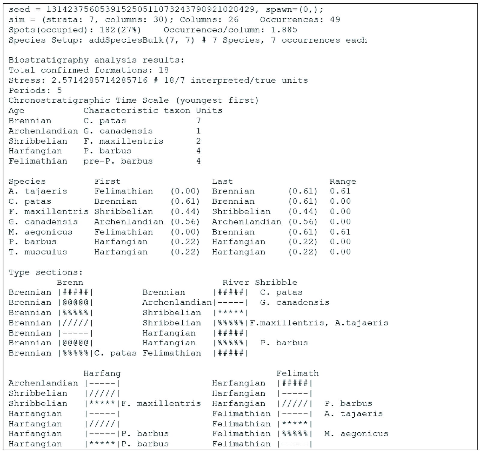
Fig. 1. Simulation output example.
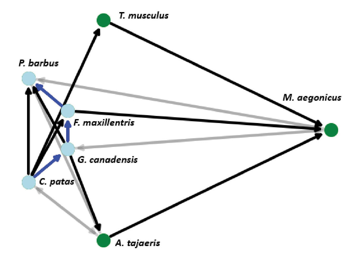
Fig. 2. A small example fossil relation network with seven taxa showing index taxa (blue circles), superposition relationships (black and blue edges with arrows), and co-occurrence relationships (gray edges).
The output below is organized into several sections. The first outputs simulation setup information including the seed, then number of strata, columns (initial and fossiliferous), species, and occurrences. The next section summarizes the results of the biostratigraphic analysis with the number of timescale periods and the number of interpreted units which are contained in them. The timescale table gives a gloss name for the period, then the characteristic taxon, and the number of formations which are represented in the period as a measure for sedimentary time lapsed. The stress is the ratio between the number of interpreted formations to the true number. The third section lists all of the species and their first and last appearances in the interpreted timescale. Index taxa by definition are restricted to their single period. The next section lists all of the relevant type sections. Each is a representation of a column, with the location name at the top. The interpreted age of each unit is on the left, followed by a representation of the lithology of each formation (this is merely a gloss, lithologies are not considered in the simulation), followed by fossil occurrences in that formation. A comparison between the timescale that results from biostratigraphic analysis and the true fossil ranges as recorded in the simulation is shown in fig. 3. In general, the biostratigraphic analysis produces an independent reconstruction that differs from the true underlying parameters.
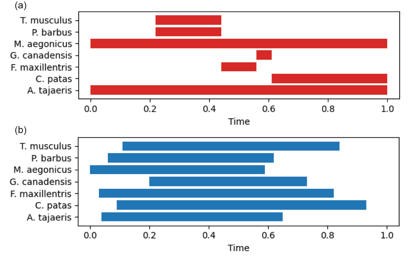
Fig. 3. Comparison between interpreted and true fossil ranges for small scale example. Timescale fraction ranges from 0 (oldest) to 1 (youngest), and is different between the interpretation and true values. Fig. 3a. Fossil ranges according to the biostratigraphic interpretation. Fig. 3b. True fossil deposition ranges as recorded by the simulation.
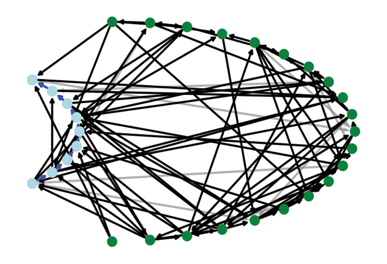
Fig. 4. Fossil relation network for a typical run with 30 taxa.
Fig. 2 shows a graph of the fossil taxa relationships in the example simulation. Solid arrows represent relations where occurrences of the taxon on the tail end are always found above (superposed) any occurrences of the head taxon whenever they are found together in the same columns. Gray, transparent arrows represent relationships between taxa where occurrences appear together in both above and below arrangements. These represent co-occurrences. Index taxa are represented with blue nodes on the left-hand side of the graph, while all other taxa are on the right. The blue arrows highlight the longest superpositional path and form the basis for the reconstructed timescale.
Fig. 4 shows an example fossil relation network from a typical large simulation run. This network size was chosen as the largest network that reliably completes analysis in a reasonable amount of time. Fossil taxa names are constructed randomly as a visual gloss, and do not correspond to actual fossil species.
Experiment descriptions
To determine the effects of the experiment parameters independent of scenario-specific variations, each experiment was run with 200 iterations, except where otherwise noted. For each iteration, the following measurements are retained for statistical analysis:
- Number of index fossils found
- Number of range extensions
- Average fossil occurrences per column
- Number of formations included in the constructed timescale
- Number of true strata—fixed at 7
- Timescale stress, defined as the number of formations in the constructed timescale divided by the true number of strata
- Network edge density
Experiment 1: Type of ordering
For this experiment, different ordering styles were compared with each other. The 150 columns in the simulation setup were divided into three geographic regions. The taxa were also divided into three cohorts and arranged as described below. Fig. 5 shows the arrangement of taxa cohorts with each represented by a primary color and overlaps represented by color mixtures, with each rectangular region being a single uniform distribution.
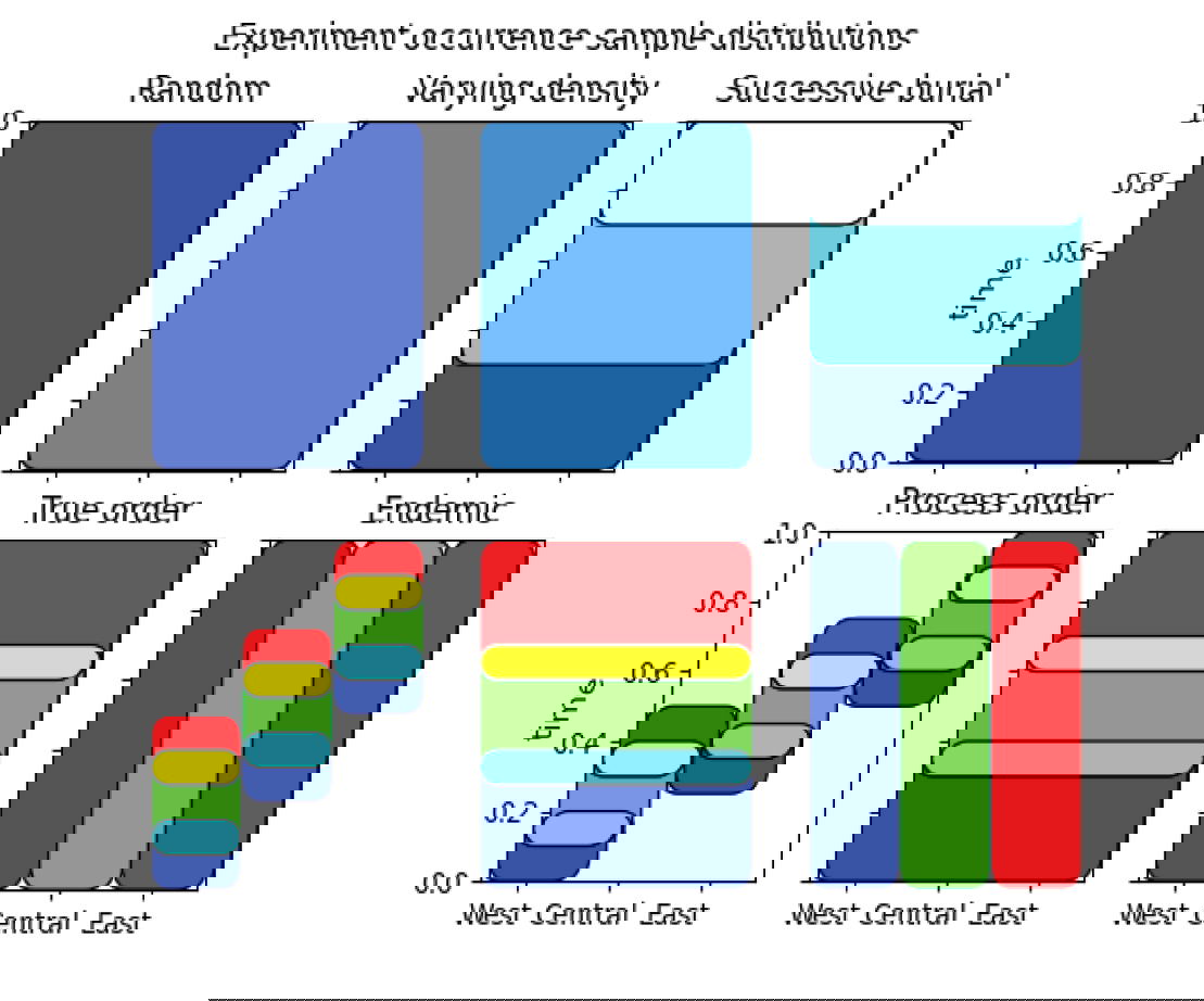
Fig. 5. Sampling distributions from which fossil occurrences are drawn with respect to time and geography for the ordering types in experiment 1.
Scenario 1: Random ordering.
In this scenario, all fossil occurrences are drawn from the same temporal uniform distribution and spread over all regions. This represents a truly random order.
Scenario 2: Varying number of fossil occurrences
This scenario is constructed in the same way as the scenario 1 random ordering, but the average density of fossil occurrences per column is allowed to vary by varying the number of columns into which occurrences are distributed per run. The same number of fossil taxa and occurrences are used for each run. The number of columns for each run is drawn from a discreet uniform distribution from 100 to 200.
Scenario 3: Successive overlapping burial
In this ordering scenario, the three fossil cohorts are distributed across all regions with the beginning time of each cohort increasing, so that the oldest cohort comes from a distribution that covers the entire time range, the second cohort covers the most recent two-thirds, and the youngest cohort is distributed in the final third. This is representative of a progressive inundation model where lower biomes are picked up before higher ones, and then all disrupted biomes are potentially buried together.
Scenario 4: Process order
This scenario is based on three cohorts which are locally truly ordered, but only cover half of the total time interval. This ordering is repeated at each location with the sequence shifted in time. In this case, local ordering should always be valid, but distant correlations will diverge from absolute time.
Scenario 5: True Order
In this scenario, the three fossil cohorts are distributed across all regions, with each cohort being drawn from distinct time ranges, which have a 25% overlap with adjacent cohorts.
Scenario 6: Endemic species
This scenario has the three fossil cohorts distributed over the entire time range, but each is restricted to a single region, to represent taxa that are endemic to single regions. This scenario was not run in the final analysis because the results were equivalent to the random order scenario with a 1/3 sample size. The additional size of the network also caused longer running times, even though each graph was partitioned into three smaller distinct communities.
Experiment 2: Successive ordering series
Another experiment was run to determine the effect of true ordering on the measured properties of timescale stress, the number of index fossils, and the number of range extensions. Similarly to scenario 5 in experiment 1 above, ordered sets of fossil cohorts were generated with 25% overlap. The number of cohorts in each scenario are: 1 (same as random ordering), 2, 3, 4, 6, 12 (fig. 6).
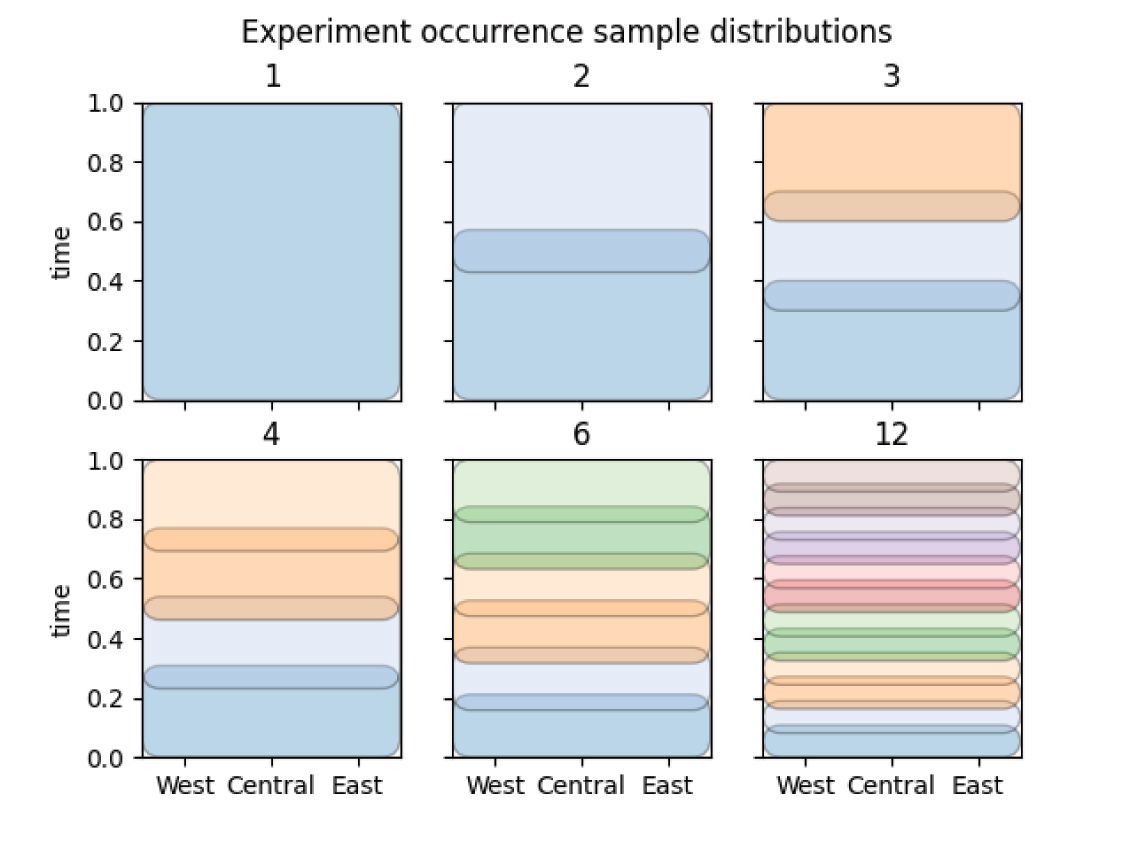
Fig. 6. Sampling distributions from which fossil occurrences are drawn in experiment 2. Each scenario has an increasing number of distributions, increasing fossil ordering.
Experiment 3: Varying fossil density
The relationship between the average fossil taxon density per column and the reliability of biostratigraphic interpretations was tested independently of ordering style like was done in Experiment 1. The total variance in occurrence density for Experiment 1 was limited by the size of the fossil relationship graph, and was not easily distinguishable from the random case. To explore the effect of higher variance a series of runs was constructed similarly to Experiment 1, but with the number of columns varied between 10 and 130. To this, occurrences of 10 taxa were added, with the number of occurrences allowed to vary according to a gamma distribution with k = 80 and θ = 1/4 with an expectation of 20 occurrences per taxon.
Results
Experiment 1
Experiment 1 tested the interpreted biostratigraphic ordering of simulated fossil records with varying real order caused by different ordering styles, including no order, true (though course) order, and two variants of partial order. Results for experiment 1 are shown in table 1 and figs. 7–10. All fossil ordering styles produced a broadly similar number of index fossils and hence biostratigraphic time divisions, regardless of how many actual divisions were present in the real ordering of the fossil record (one or three observable fossil-based divisions, depending on style with seven true lithological increments). The total number of divisions interpreted by the methodology would be the number of index fossils plus one to account for time before the first appearance of the first index fossil. The number of index fossils for both the random and the equivalent varying fossil density styles had inter-quartile range (IQR) from 10–13. Successive Burial had the fewest number of index fossils per simulation on average with an IQR of 8–10. Process Order had the tightest grouping with 10–12.5, and True Order had a broadly equivalent IQR of 9–12 index fossils (fig. 7). This result shows that a globally consistent ordering can be constructed by biostratigraphy even if there is no true underlying time ordering to fossils. Indeed, the presence and overall resolution (length) of the fossil record does not distinguish between styles of fossil order, or even no ordering at all.
| Scenario | m | b | R2 |
|---|---|---|---|
| 1 (random) | 0.351 | 1.26 | 0.582 |
| 2 (varying density) | 0.381 | 0.864 | 0.622 |
| 3 (successive burial) | 0.222 | 1.67 | 0.434 |
| 4 (process order) | 0.158 | 1.47 | 0.709 |
| 5 (true order) | 0.159 | 0.952 | 0.565 |
Table 1. Linear regression (form mx + b) for experiment 1: number of index fossils vs timescale stress.

Fig. 7. Experiment 1 results. Ordering type does not significantly impact the number of index fossils found, though Successive Burial seems to produce fewer than other order types.
Different ordering styles begin to be distinguished when looking at the timescale stress produced by the biostratigraphic analysis. Timescale stress is the ratio between the number of interpreted lithological time increments compared to the real number of lithological time increments. The effect of ordering style on the timescale stress is correlated with the style entropy. Both the random order and varying density scenarios with high entropy largely overlap, followed by successive burial, process order, and true order, the lowest entropy style. Fig. 8 plots the timescale stress for each style overall. Fig. 9 plots each scenario number of index fossils versus timescale stress. A linear regression was determined for each style, with the resulting parameters listed in table 1. Increasing ordering style entropy increases the amount of timescale expansion that each interpreted index fossil contributes to the overall timescale.
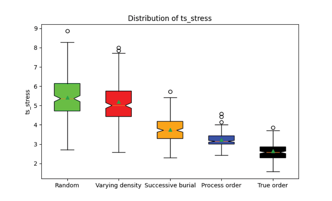
Fig. 8. Experiment 1 results. Timescale stress is strongly influenced by fossil ordering type, with stress increasing for increasing fossil disorder.
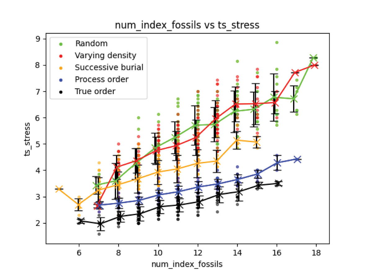
Fig. 9. Experiment 1 results. Increasing number of found index fossils increases expansion of biostratigraphic time scale. This is true even for true fossil order, though with diminished significance.
The number of range extensions expected from each of the differing ordering styles also shows a decreasing trend with increasing order (fig. 10). Random ordering produces a relatively high number of unexpected fossil orderings, which are counted as a range extension, whereas true ordering produces very few. Number of range extensions might provide an observational basis for exploring the relationship between interpreted biostratigraphic order versus true ordering for the real fossil record

Fig. 10. Experiment 1 results. Range extensions generally increase with decreasing fossil order, with process order producing the lowest number.
Experiment 2
Experiment 2 tested a series of increasingly ordered fossil records which were constructed by dividing taxa into an increasing number of time bins from which fossil occurrences were drawn. Ordering in this case is globally applicable, with a small amount of overlap between adjacent time bins. There is an effect on the overall number of index fossils based on the number of bins, though potential relationships are not well discerned from fig. 11. There appears to be a grouping of low-order divisions which have an approximately equal number of index fossils, which is larger on average than the total number of lithological divisions. The scenarios with 1 and 3 bins were included in experiment 1. The grouping on the right with a higher number of divisions representing more order appears to reach a plateau with a median number of index fossils of 7, which exactly matches the number of lithological divisions. This likely represents a form of aliasing, since in theory there should be at least as many legitimate index fossils as true time bins in the simulation. This trend is contrasting with the tendency at lower orderings to generate sequence duplications, leading to too many index fossils. These trends cut across each other, leading to the plateau behavior.

Fig. 11. Experiment 2 results. A slight decrease in number of found index fossils as fossil order increases.
In this experiment, the timescale stress measure of each scenario (fig. 12) best captures the distortion to biostratigraphically interpreted timing due to violations of the assumption of faunal succession. The totally randomly distributed scenario with only one time bin produces a large amount of timescale stress, with higher degrees of ordering asymptotically approaching the ideal stress of 1 (interpreted number of time divisions and actual number of time divisions equal).
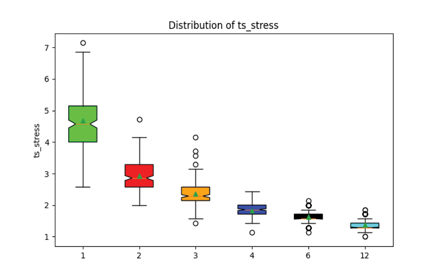
Fig. 12. Experiment 2 results. Timescale stress decreases towards 1 (no stress) with increasing fossil ordering.
Similarly to experiment 1, each simulation run was plotted with the number of index fossils against the timescale stress, and a regression analysis was performed for each number of time bins (fig. 13 with the regression analysis in table 2). The same relationship from experiment 1 where the timescale stress is proportional to the number of index fossils is evident, though the trend line becomes flatter with increasing order, represented by increasing number of fossil cohorts, indicating that highly ordered fossil records are resilient to spurious timescale extensions. The slight change in slope seen at the beginning and end of the trendlines comes from small sample sizes at those index fossil counts and is not significant.
| Cohorts | m | b | R2 |
|---|---|---|---|
| 1 | 0.327 | 1.57 | 0.541 |
| 2 | 0.196 | 1.18 | 0.558 |
| 3 | 0.19 | 0.673 | 0.556 |
| 4 | 0.0914 | 1.19 | 0.152 |
| 6 | 0.0912 | 0.929 | 0.431 |
| 12 | 0.0371 | 1.12 | 0.0182 |
Table 2. Linear regression (form mx + b) for experiment 2: number of index fossils vs timescale stress.
Fig. 13. Experiment 2 results. Increasing timescale stress with increasing length of index fossil sequence for all degrees of ordering. The slope of the correlation decreases for increasing order.
The number of range extensions for each scenario is shown in fig. 14. Range extensions decrease with increasing order to the point that in the scenario with 12 bins, runs that even had a single range extension are statistical outliers. The association between ordering and range extensions is potentially an observable that could be used to help constrain the true ordering of the real fossil record, though this could be complicated by other considerations such as paleobiogeography, and incomplete fossil preservation and collection (see discussion).
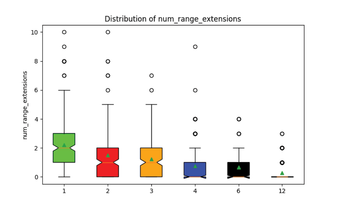
Fig. 14. Experiment 2 results. Range extensions decrease towards zero with increasing fossil ordering.
Experiment 3
Figs. 15 and 16 show the number of index fossils and timescale stress developed from a completely random fossil distribution, but with a wide range of fossil occurrence densities in columns. This leads to a densification of the number of fossil taxa associations. Both the number of index fossils interpreted and the timescale stress show a strong decline with increasing fossil density. Higher densities provide more data points into the nature of the distributions from which fossil occurrences are drawn in the form of more associations. This shows that spurious relationships that arise where all occurrences of certain taxa are always found above another, even when they are drawn from the same distribution in time, are much less common for higher fossil densities.
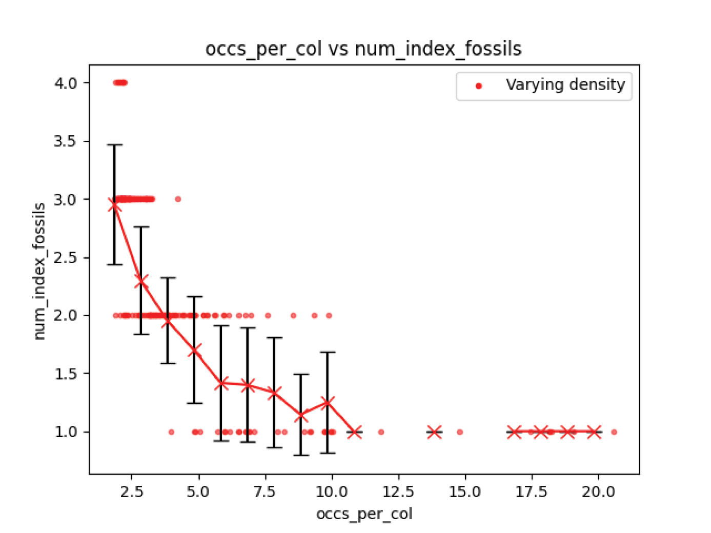
Fig. 15. Experiment 3 results. Higher fossil occurrence densities lead to lower numbers of index fossils.
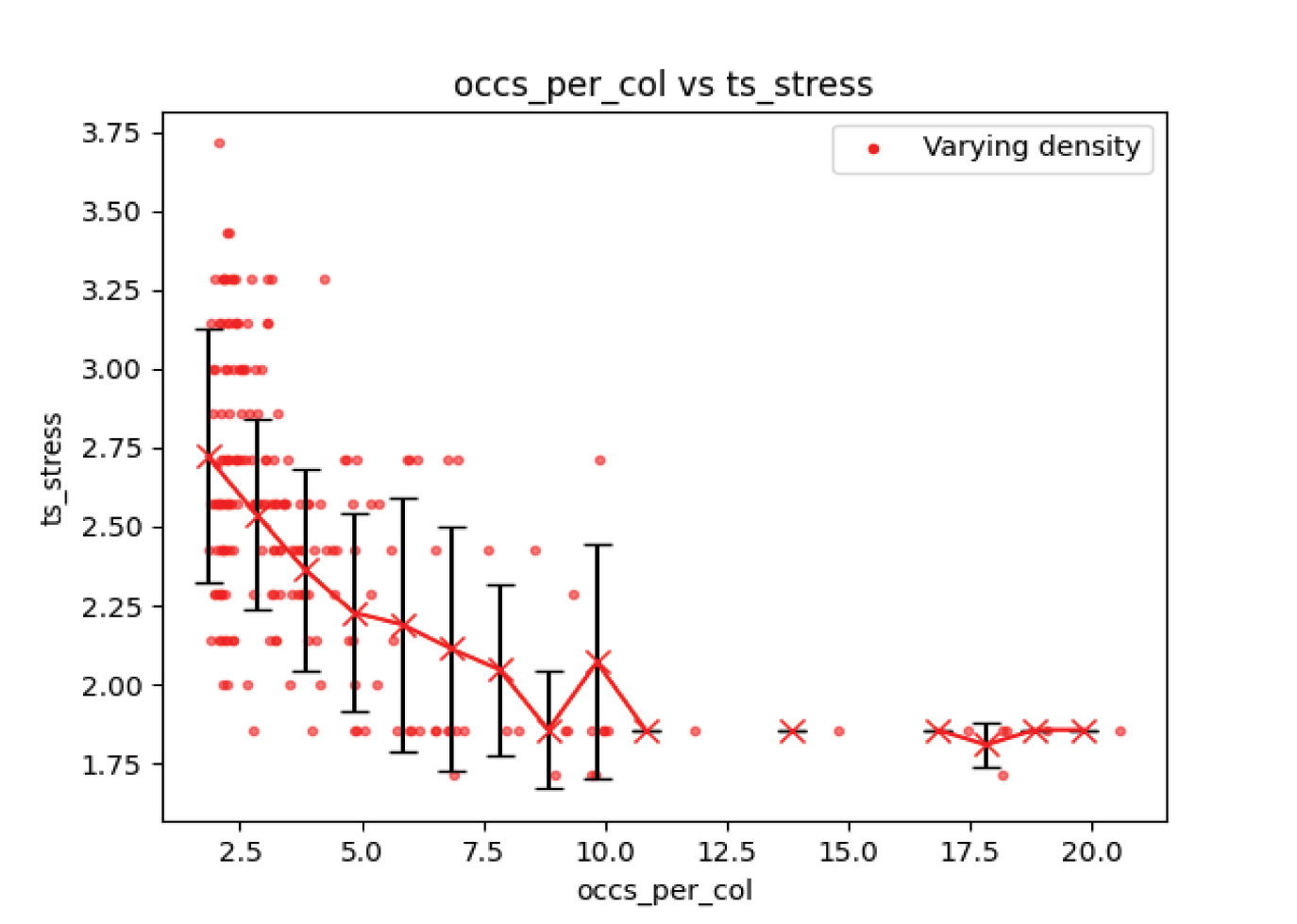
Fig. 16. Experiment 3 results. Higher fossil occurrence densities are associated with improved knowledge of the true timescale.
Discussion
The most commonly cited proof of ordering in the fossil record and the validity of biostratigraphic correlations is that it is based on empirical relationships between fossil occurrences that always hold globally. Under the standard long-age synthesis, there is also a tidy narrative of why these consistent fossil relationships have chronological significance: the evolution of a living form is unrepeatable (Dollo’s Law) and occurs at a single moment in time (faunal succession). The biblical Flood violates these assumptions and would not be expected to produce such consistent temporal fossil orderings. Subsequently, there has been much discussion on how the Flood could produce the observed fossil ordering. However, I have shown, both mathematically and by simulation, that the biostratigraphic method is guaranteed to produce an apparent time ordering from the fossil record regardless if one exists or not. Consistent fossil above/below relationships is not proof of the validity of fossil ordering!
This failure to conclusively establish order comes from us only possessing a subset of fossil associations that establish interval overlap relationships between all overlapping fossil taxa. Fossils types are not commonly found locally with the majority of other fossil types (Woodmorappe 1983). This makes it more likely for consistent relationships to arise randomly, and ensures that relative position information between arbitrary fossil pairs is sparse. This is a much more extensive knowledge gap than what is usually intended when referring to an “incomplete” fossil record, which only concerns having complete knowledge of the diversity of fossil forms. Given the sparseness of direct fossil colocations, this condition is virtually guaranteed to exist for the real fossil record. Indeed Monnet, Brayard, and Bucher (2015, 279) say that,
real data usually contain contradictions . . . which make it impossible to obtain a unique order of species ranges along the time axis.
Paleontological events are more likely to appear in contradictory order for taxa which have long true ranges or when appearance and disappearance events are closely spaced in time. This propensity for discrepancy arises due to the possibility for occurrences to be buried at any time in a long interval in the first case, and because direct associations are rare in the second case. Traditional zonal biostratigraphy typically culls these taxa from consideration for defining boundaries because of the need to find taxa and assemblages that are consistently found in the same order everywhere. The method developed in this study simulates this traditional tendency, which was used to develop the framework of the Global Chronostratigraphic Time Scale, and is still used to define Global Boundary Stratotype Section and Points (GSSPs).
Range extensions
The first and last appearances of each non-index taxon are essentially an interval hypothesis formed on the basis of the universality of the chosen timescale based on index fossils. Biostratigraphic contradictions represent a failure of that hypothesis for at least one of the taxa. The resolution of these biostratigraphic contradictions will always result in a range extension to one or more taxa. The simulation results show that increased numbers of range extensions are inversely correlated with strength of fossil ordering. Both Woodmorappe (2000) and Oard have recognized the importance of range extensions to our overall understanding of the fossil record, and have published on the ubiquity of fossil range extensions, even for well-established taxa. Oard has found enough material incidental to working on other topics, that he has maintained a semi-regular series of papers with major extensions (Oard 2009, 2010a, 2012, 2013, 2014, 2017, 2019). The two authors have reported, amongst other taxa, at least five newly discovered living fossils, two index taxa range extensions, and extensions to two major groups commonly used as index fossils. Alone, these would be merely anecdotal cases which do not necessarily represent the holistic state of the fossil record. Systematic studies on the entire fossil record show the same state of affairs. Woodmorappe (2000) cites Maxwell and Benton (1990) to show that range extensions are the normal state of affairs in vertebrate paleontology. To this, one can add a later study by Sepkoski (1993) who found that over the course of 10 years for 3,500 fossil families, 30% of all families had been redefined with 838 new families, and 199 removals. Of the remaining families, 35% of remaining families had changes in origination or extinction times. Data generally tended towards earlier origination and later extinction (that is, range extensions). Despite the numerous taxa changes, diversity patterns between the beginning and end of the study period were largely the same—indicating that any new observations can be fit into the framework despite underlying data changes. One might argue that increasing our knowledge of the evidence is the natural state of affairs, and that fossil range extensions should be the norm regardless. Not all range extensions are created equal. Merely relabeling an origination or extinction date on the basis of an external chronometer, say radiometric dating, does not really bear on the internal biostratigraphic timescale. However, when a range extension is made on a biostratigraphic basis, then it really does represent an inconsistency with the interpreted sequences. The simulations run here identify range extensions by finding the best biostratigraphic interpretation available, then integrating additional observations into that framework. The simulations show that if the framework is correct, then the new observations will generally not lead to significant range extensions. This is borne out in conventional modeling of biostratigraphy as well, which only finds minor timing distortions when faunal succession holds (Edwards 1984).
Inconsistencies in the ordering of first or last appearance events in different stratigraphic sections represent contradictions in the established biostratigraphic sequence, and are expected due to incomplete knowledge of fossil taxa ranges, even under the conventional assumptions (Sadler and Cooper 2008). Range extensions are resolved by minimizing the required adjustment to fossil taxa ranges, which is equivalent to minimizing the implied failings of the preservation and collection processes under the standard assumption of faunal succession. Without faunal succession, however, this is not the most parsimonious objective function. Many methods for finding consensus sequences (for example, simulated annealing) actually start with a random set of ranges for fossil taxa as an initial solution which trivially satisfies all possible co-occurrence constraints. The algorithm then quickly optimizes away from this initial condition based on this objective function, essentially assuming that ranges are disjoint until proven to overlap. Again, for fossils deposited during the Flood, this may not be the most parsimonious assumption.
Zero-knowledge proof
One of the reasons that consistency of fossil relations is compelling as evidence of the reality of fossil ordering is because it mimics the conditions of a probabilistic zero-knowledge proof. The classic example of a zero-knowledge proof is one in which there is a cave which has two passageways that branch off the entrance. Alice has found a pathway that connects the two pathways within the cave system. She wants to prove to Bob that she has found such a pathway, but she doesn’t want to reveal the secret to Bob to do so. To accomplish this, Alice goes into the cave down one of the two passages. Bob then calls out which passageway he would like Alice to emerge from, and she does. For a single trial, if there is no secret pathway, there is a 50% chance that Alice just happened to be hiding in the tunnel that Bob called out. The trial is repeated until Bob is satisfied to any confidence level that there really is a secret passage, and that the alternative is statistically impossible. If the fossil record were such that we could specify independently determined ordering, and then discover a global consistency of that ordering, then that would provide statistical evidence of the ordering which could be repeated with sufficient pairings to prove ordering to any level of statistical confidence. However, phylogenies of fossil taxa use the observed fossil ordering as a priori input, so they do not constitute independent trials.
The famous Monty Hall problem is an illustration of the importance of post-facto choices on the outcome of random events. The problem is named for the host of the game show “Let’s make a Deal” where a similar scenario was often featured with contestants. In the problem, the contestant picks one of three doors which conceal prizes, one of which is a high-value prize with the others concealing low-value “zonk” prizes. Monty then reveals a zonk from one of his remaining two doors, then offers to trade doors with the contestant. The often-unintuitive best strategy for the contestant in this situation is to make the trade, as the grand prize has a 2/3 chance of being behind the Monty’s door, and only 1/3 chance of being behind the door initially selected. The reason for this is that Monty makes his selection of which door to reveal after the contestant has selected, and he will not choose to reveal the grand prize—so the selected revealed door is not independent of the contestant’s choice, so does not change the probability of the contestant’s door hosting the grand prize from the initial guess.
By contrast, consider a slight modification to the game where there are three distinct prize values, and the host’s strategy for revealing the door is based on a coin flip, rather than prior knowledge about where the grand prize is. In this case, there is a 1/3 chance that Monty will reveal the grand prize before asking the contestant to switch, and there is now equal probability for the greater of the two remaining prizes to be behind either remaining door.
Analogously, the biostratigrapher’s choice of index intervals is not made independently of the known fossil pairwise orderings. Those choices will be consistent with the observed orderings so will not add independent information about the underlying process which produced the orderings. A different potential “choice” of observed orderings by the same underlying process would still produce a coherent stratigraphic scheme even while potentially differing from the first case.
Timing considerations
There are 79 Phanerozoic + Ediacaran “ages” below the K-Pg boundary in the uniformitarian geologic timescale (Cohen, Harper, and Gibbard 2024). Assuming that each of these proceeded in sequence, and that they were laid down over 371 days during the year of the Flood, then the average deposition time for each age would be 4.7 days. If the period of time during the Flood representing preserved deposition were shorter, or the number of ages deposited by the Flood were greater, then that average could be as low as 1.5 days. Biostratigraphy is often performed to even finer scales of gradation. If one were to further divide two ages into nine subintervals (as was done by Ross 2009), then each of those subintervals would average at most 25 hours and three minutes long. The implication of valid time ordering of biostratigraphic correlations is that all occurrences of taxa that are confined to one of these biostratigraphic subintervals would need to be deposited on the exact same day—and only that day, despite deposition localities being separated by hundreds to thousands of miles. The situation is even worse for ammonoids, which are the primary group used for defining interval biozones in the Mesozoic. The same period of time subdivided into the 37 ammonite (Lehmann 2015) and triceratops (late Maastrichtian, Lehman 1987) zones would mean a new taxon would need to be buried for the first time globally, and then complete burial of all members of that taxon within six hours and five minutes on average. This would only be reasonable during the Flood for taxa that have very provincial distributions—sub-regional at the most.
Most YEC models of generating fossil ordering do not have a narrative sufficient for explaining fossil ordering so tightly, and it does not arise deductively from the core postulates of the models. This is true in part, because ecological zonation, and escape mobility separate out creatures by their time of inundation, not their final deposition. Hydrodynamic sorting and Tectonically Associated Biological provinces (TABs) potentially could supply global timing constraints on deposition, but these are not currently popular as the main agents of fossil ordering. In light of the results presented here, it may not be necessary for these ordering models to account for this strict global timing as even a fairly large distortion from strict timing can potentially present the same ordering evidence.
Independent tests of time significance of Ordering
True fossil time ordering may still exist, since a set of consistent relationships is a necessary condition for temporal ordering, but we do not at this time have an independent test to determine to what extent observed fossil ordering is real or spurious. Finding a test is critical because it helps us to better understand the dynamics of the Flood, enables biostratigraphy to be used as a distinguishing criterion between the Flood and Antediluvian and Modern eras (Whitmore and Garner 2008), and can be used as expected as a timing indicator in the post-Flood era.
Independent chronometers
The most obvious test for true ordering would be to compare ordering results with another independent chronometer. There are two primary candidates, magnetostratigraphy (polarity chronology) and radiometric dating. Sedimentary rocks can be measured to determine the polarity and strength of the earth’s magnetic field near the time of deposition. Changes to the polarity can be mapped vertically through the sedimentary column and horizontally from basin to basin. These changes represent isochronous points in time—that is, they change simultaneously all over the earth. Unfortunately, one normal polarity reading cannot be distinguished from another when the record is physically discontinuous. Only the ocean basins contain an unbroken record of magnetic field polarity reversals, and even then, the timing of each event and the rate of reversals cannot be determined without external timing controls. For terrestrial locations, only a small handful of reversals are typically preserved, so the observed transitions have to be fit into the global polarity timescale via an external time marker. The time marker initially used to do the fitting is—you guessed it—biostratigraphy. So, without significant reanalysis, magnetostratigraphy is not independent of biostratigraphy and cannot be the external time witness.
Radiometric dating is the only remaining possible independent time measure. The RATE study showed that radiometric methods have the potential for constraining relative ages (Vardiman, Snelling, and Chaffin 2005). However, there are a few potential issues. Firstly, fossils are generally not contained in rocks that can be directly radiometrically dated. In many cases, fossil ages can be bracketed above and below by rocks that can be dated or detrital grains, though only in the most ideal cases is this able to provide very tight timing control. Such high-quality control would need to be obtained systematically to constrain ordering in the general case. Secondly, radiometric dates have noise and can be affected by the thermal and decay history of rocks. This limits the precision of relative dating between differing localities, and may prevent verification of highly specific biostratigraphic schemes, for example, the appearance of individual species of a genus. Modern dating techniques have largely eliminated the variance in dating arising from the dating methods themselves, which was a significant and common in the early decades of radiometric methods (Hu et al. 2018; Kelley 2002). Thirdly and most significantly, accelerated nuclear decay causes systematic effects that are geographically linked, which complicates the direct comparison of geographically separated radiometric dates, even if other more commonly addressed issues like thermal histories are non-factors (Mogk 2023). To fully utilize radiometric dating for validation of fine-scale biostratigraphic order, a complete picture of local systematic factors should be determined as suggested in Mogk (2023). Until then, his relative dating condition number 3 (Mogk 2023, 333) might be used. The analysis done by Woodmorappe (1979) which directly compared radiometric dates to biostratigraphic determinations found that rocks from individual periods could be measured over a range of about 250M radiometric years. This suggests a minimum required separation based on the radiometric dates available at the end of the 1970s. Further research with modern radiometric data might be able to constrain an acceptably narrow separation which accounts for all uncertainties.
Globally identifiable isochronous events
If other isochronous events during the Flood can be identified, then they can be used to constrain actual fossil ordering, though the granularity will be limited to the number of events identified—possibly only a few total gradations. To provide global time control, such isochronous events would need to be globally identifiable. Impact events with stratigraphic markers would make good candidates. Megasequence boundaries may also prove promising.
Stratomorphic series
A stratomorphic series consists of taxa which constitute a trend of morphological intermediates in stratigraphic succession (Wise, 1995). Stratomorphic series are expected to reflect the post-Flood fossil record of diversification from surviving forms, however they are expected to be rare in Flood sediments. Therefore, one might suppose that stratomorphic series could be a test of the validity of temporal ordering in fossils consisting of a sufficiently long sequence of taxa that can be related to each other in multiple locations.
Differences in the existence and validity of stratomorphic series could be used to test the location of the Flood/post-Flood boundary (Doran, Garner, and McLain 2021). Indeed, the horse stratomorphic series has been used as evidence of the Cenozoic being post-Flood (Cavanaugh, Wood, and Wise 2003). However, there are numerous stratomorphic series in taxa who are buried exclusively in sediments that are widely considered to have been laid down during the Flood, including cynodonts (Lay and McLain 2019), Ornithomimosauria (Doran and McLain 2021), Anklysauria (Doran and McLain 2022), and others (Doran, Hartman, and Sanderson 2018). Any true stratomorphic series which is preserved in Flood sediments must be due to some sort of process separation, whether or not that process also results in real timing differences in the burial of various taxa. Without a better understanding of the nature of those processes which can produce stratomorphic series during the Flood, it is difficult to differentiate series produced diachronously by such processes from one produced by diversification and dispersal through time.
Given the timing distortions implied by this study, it may be difficult to identify Flood deposited stratomorphic series by first appearance datum (FAD)/last appearance datum (LAD) data alone. An external source of information to establish a seriation expectation would be required to compare to the apparent fossil order, like phylogenetic sequences. The existence of this type of ordering in the fossil record was examined by McGuire et al. (2023) who found that the expected ordering of most phylogenies do not correlate well with the observed biostratigraphic ordering. This is also true of conventional studies which attempted to test the ordering of the fossil record with a similar methodology (Benton and Storrs 1994), which showed that 45% of cladograms matched the expected phylogeny at p < 0.05 significance, and only 25% of phylogenies were significant at p < 0.01.
Distant taxon-strata correspondences
Another possible test of true temporal ordering is if particular taxa are associated in different regions with particular identifiable lithological strata (for example, chalk). If the strata can indeed be shown to be coeval at the distant locations, then this would provide an independent means of establishing relative time, at least in the regions where this can be demonstrated. However, this requirement may be more difficult to achieve in practice than one might assume for Flood deposited sediments. The standard stratigraphic principles of superposition, lateral continuity, and original horizontality treat strata as synchronous deposits under the assumption that the time taken to deposit the extent of a stratum is much less than the time taken to deposit its thickness. If the time taken is equivalent, or if the thickness is deposited faster than the extent, then the stratum will be diachronous. Essentially all rocks deposited by the Flood will be diachronous due to the violation of this assumption. This can be shown as the average depositional rate during the Flood is as high as 27 ft per day. A formation like the Coconino Sandstone might take 12 days to accumulate, but 2.5–10 days for the depositing current to traverse the known area of outcrops (Helble 2011). This means that it is possible that the upstream end of the deposit was nearly completely deposited before the most distal downstream end had received its first grains. The isochrone surface within the sediments of such strata is tilted, with deposition proceeding laterally as well as vertically, as has been shown in laboratory flume experiments (Julien, Lan, and Berthault 1993).
Combinatorial completeness test
In the absence of a suitable independent chronometer, a test for the completeness of all possible fossil pairings for a given defined faunal assemblage may be sufficient to establish the validity of sequences arising in that particular assemblage. Sadler and Cooper (2008) examined the ratio of contradictory sequences of pairs of events against the number of stratigraphic sections examined, where an event pairing was considered contradictory if both sequences of the events (that is, A-before-B and B-before-A) were observed in separate sections. They only looked at pairings of taxa whose ranges are known to overlap including Ordovician through early Devonian graptolites and Late Miocene to Recent foraminifera and radiolaria. As additional sections were examined, the contradiction ratio tended towards 1, though the authors claim that the growth was lower than that expected if the odds of contradiction were constant for every pair of events. They offer the suggestion that some pairs are easier to record in contradictory order, presumably because of real separations between taxa preserved in the fossil record. Such separations could be caused by true time ordering or process ordering, and could possibly be inverted to detect random intervals.
Distortion of event timing
The timing distortions which generate the timescale stress and duplication manifest in each local column as a stretching and compression of time which overall maintains the local ordering of events. However, when different columns are integrated, intervals of time become multiplied, leading to the potentially high values of timescale stress as observed in the simulation. Truly synchronous events also become duplicated and can appear to occur at differing times in the constructed timescale depending on the location examined.
Paleontological data have never been more accessible to research given the rise of public databases that attempt to include the entirety of the published literature. At the time of this writing (November 2024), PaleoBioDB contains 89,611 references and 1,625,087 individual fossil occurrences, and more are regularly added. The database also provides a variety of tools for accessing and visualizing the data. The PaleoBioDB represents an accurate picture of the published literature at the time of its original publication, and does not attempt to normalize timing constraints between occurrences. Age control can range from biostratigraphic only, to well-bracketed by high precision radiometric dates, depending on what was available at the time of publication as well as the purpose of the individual study. The degree to which adopted ages are affected by timescale stress will vary from study to study, with also likely variations according to publication year depending on the tools and methods that were available at that time.
The dozens of papers which use biostratigraphic position as their sole timing control are potentially subject to distortions, particularly when relying on finer biostratigraphic divisions.
Conclusions and Future Studies
Zeller (1964) showed that both correlations of sections and interpretation of cyclicity could be made for sequences that had been generated from completely random data—a result of our need to find order in the world around us which can potentially lead to biased interpretations of data. While not suggesting that correlations are phantasms of the human mind, Zeller did exhort his readers to distinguish random events versus the necessary consequences of events, which are non-random. This study showed that spurious stratigraphies can be made from entirely randomly ordered fossil occurrence data. The association of fossils with particular strata, in relation to one another is an empirical reality, but that this corresponds to a temporal sequence is an assumption that cannot be established by the fossil association data alone. The reasons for this are:
- The Flood conditions directly abrogate the assumption of Faunal Succession.
- The overall fossil sequence is fit posteriorly to observations, and is not well predicted by any described mechanisms.
- Observed associations between arbitrary pairs of fossils are mathematically sparse. Co-occurrence is the only relation that can be conclusively determined from fossil relationships. Biostratigraphy usually explicitly assumes temporal separation if a co-occurrence is not observed. That is, absence of evidence used as evidence of absence.
- Strata laid down during the Flood are diachronous.
When given appropriate conditions which will necessarily produce faunal succession, then fossil correlations will correspond to true time sequences. However, in the absence of a sufficient cause, then biostratigraphic interpretations can be entirely spurious.
For Flood-deposited strata, the implications of this study are potentially significant. It is likely that the interpreted ordering of the fossil record is more apparent than real. The degree to which ordering actually exists in the fossil record and to what precision biostratigraphy can be performed must be independently established by additional time markers. As a significant percentage of geological data is indexed according to biostratigraphic time correlations, this work could significantly impact how we understand geological events and causality in the Flood, paleobiogeography, and the post-Flood boundary.
One might say that because the global biostratigraphic column was first developed in Europe, and then applied to other continents and found to work that constitutes proof that the sequence is real and globally valid. A future study will simulate this scenario and assess the likelihood of being able to construct valid biostratigraphic sequences serially across continents that are analogous with the historical development of the biostratigraphic column. Other future studies will replicate the results of this paper with conventional computational biostratigraphy tools like UA-graph, developing and evaluating the ordering statistics proposed in this paper and others on high-quality biostratigraphic datasets (such as those referenced in Sadler and Cooper 2008), and simulating fossil diversity scenarios (for example, species bottleneck) on interpreted timescales.
References
Benton, M. J. and G. W. Storrs. 1994. “Testing the Quality of the Fossil Record: Paleontological Knowledge is Improving.” Geology 22, no. 2 (February 1): 111–114.
Burdick, Clifford L. 1976. “What About the Zonation Theory?” Creation Research Society Quarterly 13, no. 1 (June): 37–38.
Cavanaugh, David P., Todd Charles Wood, and Kurt P. Wise. 2003. “Fossil Equidae: A Monobaraminic, Stratomorphic Series.” In Proceedings of the Fifth International Conference on Creationism. Edited by R. L. Ivey, Article 11. Pittsburgh, Pennsylvania: Creation Science Fellowship.
Clark, Harold Willard. 1946. The New Diluvialism. Angwin, California : Science publications.
Clark, Harold W. 1971. “Paleoecology and the Flood.” Creation Research Society Quarterly 8, no. 1 (June): 19–23.
Clark, Harold W. 1977. “Fossil Zones.” Creation Research Society Quarterly 14, no. 2 (September): 88–91.
Cohen, K., D. Harper, and P. Gibbard. 2024. “ICS International Chronostratigraphic Chart 2024/12.” International Commission on Stratigraphy, IUGS. www.stratigraphy.org.
Cutler, Alan H., and Karl W. Flessa. 1990. “Fossils Out of Sequence: Computer Simulations and Strategies for Dealing with Stratigraphic Disorder.” Palaios 5, no. 3 (June): 227–235.
Darwin, C. 1859. On the Origin of Species: A Facsimile of the First Edition. Cambridge, Massachusetts: Harvard University Press.
Doran, N. A., P. Garner, and M. A. McLain. 2021. “Understanding Stratomorphic Series.” Journal of Creation, Theology and Science, Series B: Life Sciences 11: 2–3.
Doran, Neal A., Matthew A McLain, N. Young, and A. Sanderson. 2018. “The Dinosauria: Baraminological and Multivariate Patterns.” In Proceedings of the Eighth International Conference on Creationism. Edited by J.H. Whitmore, 404–457. Pittsburgh, Pennsyvlania: Creation Science Fellowship.
Doran, N. A., and M. A. McLain. 2021. “The Ornithomimosauria Holobaramin in Stratigraphic Perspective.” Journal of Creation, Theology and Science, Series B: Life Sciences 11: 3–4.
Doran, N. A., and M. A. McLain. 2022. “The Ankylosauria: A Bottom-Heavy Holobaramin?” Journal of Creation, Theology and Science, Series B: Life Sciences 12: 3–4.
Edwards, Lucy E. 1984. “Insights on Why Graphic Correlation (Shaw’s Method) Works.” The Journal of Geology 92, no. 5 (September): 583–597.
Gibson, L. James. 1996. “Fossil Patterns: A Classification and Evaluation.” Origins 23, no. 2 (June 1): 68–99.
Guex, Jean. 2011. “Some Recent ‘Refinements’ of the Unitary Association Method: A Short Discussion.” Lethaia 44, no. 3 (8 July): 247–249.
Guex, Jean, and Eric Davaud. 1984. “Unitary Associations Method: Use of Graph Theory and Computer Algorithm.” Computers and Geosciences 10, no. 1: 69–96.
Helble, Timothy K. 2011. “Sediment Transport and the Coconino Sandstone: A Reality Check on Flood Geology.” Perspectives on Science and Christian Faith 63, no. 1 (March): 29–41.
Holland, Steven M. 2000. “The Quality of the Fossil Record: A Sequence Stratigraphic Perspective.” Paleobiology 26, no. S4:148–168.
Holland, Steven M. 2003a. “BIOSTRAT: A Program for Simulating the Stratigraphic Occurrence of Fossils.” Computers and Geosciences 29, no. 9 (November): 1119–1125.
Holland, Steven M. 2003b. “Confidence Limits on Fossil Ranges That Account for Facies Changes.” Paleobiology 29, no. 4 (Autumn): 468–479.
Holland, Steven M., and Mark E. Patzkowsky. 1999. “Models for Simulating the Fossil Record.” Geology 27, no. 6 (June 1): 491–494.
Holland, Steven M., and Mark E. Patzkowsky. 2002. “Stratigraphic Variation in the Timing of First and Last Occurrences.” PALAIOS 17, no. 2 (April): 134–146. CO;2.
Hu, Rong-Guo, Xiu-Juan Bai, Jan Wijbrans, Fraukje Brouwer, Yi-Lai Zhao, and Hua-Ning. Qiu. 2018. “Occurrence of Excess 40Ar in Amphibole: Implications of 40Ar/39Ar Dating by Laser Stepwise Heating and in vacuo Crushing.” Journal of Earth Science 29, no. 2 (17 April): 416–426.
Johnson, Noye M., Neil D. Opdyke, and Everett H. Lindsay. 1975. “Magnetic Polarity Stratigraphy of Pliocene-Pleistocene Terrestrial Deposits and Vertebrate Faunas, San Pedro Valley, Arizona.” Geological Society of America Bulletin 86, no. 1 (January 1): 5–12.
Julien, Pierre, Yongqiang Lan, and G. Berthault. 1993. “Experiments on Stratification of Heterogeneous Sand Mixtures.” Bulletin Societe Géologique De France 164, no. 5: 649–660.
Kelley, Simon. 2002. “K-Ar and Ar-Ar Dating.” Reviews in Mineralogy and Geochemistry 47, no. 1: 785–818.
Lay, A., and M. A. McLain. 2019. “Preliminary Results from Reanalyzing the Cynodont to Mammal Transitional Sequence.” Journal of Creation, Theology and Science Series B: Life Sciences 9: 3–4.
Lehman, Thomas M. 1987. “Late Maastrichtian Paleoenvironments and Dinosaur Biogeography in the Western Interior of North America.” Palaeogeography, Palaeoclimatology, Palaeoecology 60: 189–217.
Lehmann, J. 2015. “Ammonite Biostratigraphy of the Cretaceous—An Overview.” In Ammonoid Paleobiology: From Macroevolution to Paleogeography. Edited by Christian Klug, Dieter Korn, Kenneth De Baets, Isabelle Kruta, and Royal H. Mapes, 403–429. Heidelberg, Germany: Springer.
Lindsay, Everett H., Gary A. Smith, C. Vance Haynes, and Neil D. Opdyke. 1990. “Sediments, Geomorphology, Magnetostratigraphy, and Vertebrate Paleontology in the San Pedro Valley, Arizona.” The Journal of Geology 98, no. 4 (July): 605–619.
Maxwell, W. Desmond, and Michael J. Benton. 1990. “Historical Tests of the Absolute Completeness of the Fossil Record of Tetrapods.” Paleobiology 16, no. 3 (Summer): 322–335.
McGuire, Kathryn, Sophie Southerden, Katherine Beebe, Neal Doran, Matthew McLain, Todd Charles Wood, and Paul A. Garner. 2023. “Testing the Order of the Fossil Record: Preliminary Observations on Stratigraphic-clade Congruence and Its Implications for Models of Evolution and Creation.” In Proceedings of the Ninth International Conference on Creationism. Edited by J. H. Whitmore: 478–488. Cedarville, Ohio: Cedarville University.
Mogk, Nathan. 2023. “Tapping the Hourglass: Disequilibrium Relaxation Following Accelerated Nuclear Decay.” In Proceedings of the Ninth International Conference on Creationism. Edited by J. H. Whitmore: 327–345. Cedarville, Ohio: Cedarville University.
Mogk, Nathan W. 2025. “Simulating Biostratigraphy to Test Faunal Succession.” Answers Research Journal 18 (October 15): 487–495. https://answersresearchjournal.org/fossils/simulating-biostratigraphy-faunal-succession/.
Monnet, Claude, Arnaud Brayard, and Hugo Bucher. 2015. “Ammonoids and Quantitative Biochronology—A Unitary Association Perspective.” In Ammonoid Paleobiology: From Macroevolution to Paleogeography. Edited by Christian Klug, Dieter Korn, Kenneth De Baets, Isabelle Kruta, and Royal H. Mapes, 277–298. Heidelberg, Germany: Springer.
Monnet, Claude, Christian Klug, Nicolas Goudemand, Kenneth De Baets, and Hugo F. R. Bucher. 2011. “Quantitative Biochronology of Devonian Ammonoids from Morocco and Proposals for a Refined Unitary Association Method.” Lethaia 44, no. 4 (February): 469–489.
North American Commission on Stratigraphic Nomenclature. 2005. “North American Stratigraphic Code.” AAPG Bulletin 89, no. 11 (November): 1547–1591.
Oard, Michael J. 2009. “Evolutionary Fossil-Time Ranges Continue to Expand.” Journal of Creation 23, no. 3 (December): 14–15.
Oard, Michael J. 2010a. “Further Expansion of Evolutionary Fossil Time Ranges.” Journal of Creation 24, no. 3 (December): 5–7.
Oard, Michael J. 2010b. “The Geological Column is a General Flood Order with Many Exceptions.” Journal of Creation 24, no. 2 (August): 78–82.
Oard, Michael J. 2012. “Fossil Ranges Continue to Expand.” Journal of Creation 26, no. 1 (April): 15–16.
Oard, Michael J. 2013. “Fossil Range Extensions Continue.” Journal of Creation 27, no. 3 (December): 79–83.
Oard, Michael J. 2014. “Fossil Time Ranges Continue to be Increased.” Journal of Creation 28, no. 3 (December): 3–4.
Oard, Michael J. 2017. “Fossil Time Ranges Continue to Expand Up and Down.” Journal of Creation 31, no. 2 (August): 3–5.
Oard, Michael J. 2019. “More Expansion of Fossil Time Ranges.” Journal of Creation 33, no. 3 (December): 3–4.
Opdyke, N. D., E. H. Lindsay, N. M. Johnson, and T. Downs. 1977. “The Paleomagnetism and Magnetic Polarity Stratigraphy of the Mammal-Bearing Section of Anza Borrego State Park, California.” Quaternary Research 7, no. 3 (May): 316–329.
Opdyke, Neil D., and James E. T. Channell. 1996. “Cenozoic Terrestrial Magnetic Stratigraphy.” International Geophysics 64: 144–167.
Peters, Shanan E., and Michael McClennen. 2016. “The Paleobiology Database Application Programming Interface.” Paleobiology 42, no. 1 (23 December): 1–7.
Price, George McCready. 1923. The New Geology. Mountain View, California: Pacific Press Publishing Association.
Puolamäki, Kai, Mikael Fortelius, and Heikki Mannila. 2006. “Seriation in Paleontological Data Using Markov Chain Monte Carlo Methods.” PLoS computational biology 2, no. 2:e6.
Reed, John K. 2008. “Toppling the Timescale—Part II: Unearthing the Cornerstone.” Creation Research Society Quarterly 44, no. 4 (Spring): 256–263.
Robinson, Steven J. 1996. “Can Flood Geology Explain the Fossil Record?” Creation Ex Nihilo Technical Journal 10, no. 1 (April): 32–69.
Ross, Marcus R. 2009. “Charting the Late Cretaceous Seas: Mosasaur Richness and Morphological Diversification.” Journal of Vertebrate Paleontology 29, no. 2: 409–416.
Ross, Marcus R. 2012. “Evaluating Potential Post-Flood Boundaries with Biostratigraphy—the Pliocene/Pleistocene Boundary.” Journal of Creation 26, no. 2 (August): 82–87.
Sadler, Peter M. and Roger A. Cooper. 2008. “Best-Fit Intervals and Consensus Sequences.” In High-Resolution Approaches in Stratigraphic Paleontology. Topics in Geobiology. Vol. 21. Edited by P. J. Harries, 50–94. New York, New York: Springer.
Sepkoski, J. J. Jnr. 1993. “Ten Years in the Library: New Data Confirm Paleontological Patterns.” Paleobiology 19, no. 1 (Winter): 43–51.
Shaw, Alan B. 1964. Time in Stratigraphy. Vol. 1. New York, New York: McGraw-Hill.
Smith, William. 1817. Stratigraphical System of Organized Fossils with Reference to the Specimens of the Original Geological Collection in the British Museum: Explaining Their State of Preservation and Their Use in Identifying the British Strata. Vol. 1. London, United Kingdom: E. Williams.
Tosk, Tammy. 1988. “Foraminifers in the Fossil Record: Implications for an Ecological Zonation Model.” Origins 15, no. 1 (January 1): 8–18.
Valentine, James W., David Jablonski, Susan Kidwell, and Kaustuv Roy. 2006. “Assessing the Fidelity of the Fossil Record by Using Marine Bivalves.” Proceedings of the National Academy of Sciences 103, no. 17 (April 25): 6599–6604.
Vardiman, Larry, Andrew A. Snelling, and Eugene F. Chaffin (eds). 2005. Radioisotopes and the Age of the Earth: Results of a Young-Earth Creationist Research Initiative. El Cajon, California: Institute for Creation Research and Chino Valley, Arizona: Creation Research Society.
Whitcomb, John C., and Henry M. Morris. 1961. The Genesis Flood. Grand Rapids, Michigan: Baker Book House.
Whitmore, John H., and Paul Garner. 2008. “Using Suites of Criteria to Recognize Pre-Flood, Flood, and Post-Flood Strata in the Rock Record with Application to Wyoming (USA). In Proceedings of the Sixth International Conference on Creationism. Edited by Andrew A. Snelling, 425–448. Pittsburgh, Pennsylvania: Creation Science Fellowship; Dallas, Texas: Institute for Creation Research.
Wise, Kurt P. 1995. “Towards a Creationist Understanding of ‘Transitional Forms’.” Creation Ex Nihilo Technical Journal 9, no. 2 (August): 216–222.
Wise, Kurt P. 2003a. “The Hydrothermal Biome: A Pre-Flood Environment.” In Proceedings of the Fifth International Conference on Creationism. Edited by R. L. Ivey, 359–370. Pittsburgh, Pennsylvania: Creation Science Fellowship.
Wise, Kurt P. 2003b. “The Pre-Flood Floating Forest: A Study in Paleontological Pattern Recognition.” In Proceedings of the Fifth International Conference on Creationism. Edited by R. L. Ivey, 371–381. Pittsburgh, Pennsylvania: Creation Science Fellowship.
Woodmorappe, John. 1979. “Radiometric Geochronology Reappraised.” Creation Research Society Quarterly 16, no. 2 (September): 102–129.
Woodmorappe, John. 1983. “A Diluviological Treatise on the Stratigraphic Separation of Fossils.” Creation Research Society Quarterly 20, no. 3 (December): 133–185.
Woodmorappe, John. 2000. “The Fossil Record: Becoming More Random All the Time.” Creation Ex Nihilo Technical Journal 14, no. 1 (April): 110–116.
Zeller, Edward J. 1964. “Cycles and Psychology.” Geological Survey of Kansas Bulletin 169 (December): 631–636.
Zhang, Tao, and Roy E. Plotnick. 2006. “Graphic Biostratigraphic Correlation Using Genetic Algorithms.” Mathematical Geology 38 (October): 781–800.