

Research conducted by Answers in Genesis staff scientists or sponsored by Answers in Genesis is funded solely by supporters’ donations.
Abstract
I analyze Walt Brown’s determination of the date of the Flood within his hydroplate model using the orbits of two comets. Brown’s result is an unwarranted extrapolation of data gleaned from the literature. The uncertainty in the data expressed by the authors of that data show that Brown’s result is unjustified, and hence Brown’s statistical analysis is meaningless. The results of this determination of the date of the Flood highly depend upon the assumed ephemerides of the two comets. There is a considerable uncertainty in those ephemerides when extrapolated so far into the past, so this method to establish the date of the Flood is not possible.
Keywords: date of the Flood, comets, hydroplate model, perihelion, ephemerides
Introduction
According to the hydroplate model (Brown 2008), God created the earth with large subterranean chambers filled with water. These water-filled chambers date to Day Two of the Creation Week, as they were the waters below the firmament made on that day (Genesis 1:6–8). In the time between the creation and the Flood, pressure built up in the subterranean chambers so that they burst forth at the beginning of the Flood. Brown identifies the eruption of the subterranean water with the fountains of the great deep (Genesis 7:11) as the primary source of water for the Flood. Some of this erupted water remained on the earth to provide large amounts of rain. However, according to the hydroplate model, a portion of the water escaped the earth, along with entrained rock and other debris. This material eventually coalesced into asteroids and comets. Previously, I have evaluated astronomical aspects of the hydroplate model and found the model wanting, particularly with regard to this proposal for the origin of comets (Faulkner 2013).
Using his hydroplate model, Brown recently proposed a method of astronomically dating the Flood (Brown 2014). If all comets were ejected from the earth at the time of the Flood as his hydroplate model proposes, then one might expect that all comets would have been in the earth’s vicinity at the time of the Flood. Using known orbital parameters of comets, we can compute the positions of comets into the past. There is a wide range in the orbital parameters of comets, including their periods. Having such a wide range in orbital periods, any two comets will infrequently return to the earth’s vicinity and hence be near to their point of origin at the same time. Therefore, if one were to compute backward in time to identify an epoch when two or more comets coincidentally were near the earth, that epoch might identify the time of the Flood. Comets move very rapidly when near perihelion, the point of closest approach to the sun, but move much more slowly when far from perihelion. Thus, comets spend only a small fraction of their orbital periods near perihelion and hence spend most of the time far from perihelion. Comet perihelia lie close to the earth’s orbit, so closest approach of a comet to both the earth and the sun are approximately coincident. Therefore, within Brown’s methodology, computing time of past perihelion passage of a comet is sufficiently coincident with the comet’s closest pass to earth. Brown used this methodology to conclude a probable date of the Flood in the year 3290 BC ± 100 years. He also claimed this result as confirmation of his hydroplate theory. This date for the Flood is at variance with the Ussher date (2349 BC). Ussher used the Masoretic text; if one uses the chronology of the Septuagint (LXX), the date of the Flood was much earlier. Brown’s astronomically determined date of the Flood is consistent with a biblical date derived from the LXX. Brown (Brown 2008, pp. 380–381) previously favored the Ussher date, and apparently still does (Brown 2015), though his astronomically determined date may have begun to change his thinking on this (Brown 2014).
As straightforward as this calculation may seem, there are two complicating factors. First, comets do not follow orbits that are governed strictly by gravity. Rather, comets exhibit slight discrepancies from orbits described by Newtonian gravity alone. The differences between the observed trajectories of comets from those predicted by Newtonian gravity probably are due to outgassing of material that acts as jets. Comet nuclei have relatively low mass, so these jets push comet nuclei slightly from the trajectories that they would otherwise follow due to gravity alone. These discrepancies are most pronounced near, but especially shortly after, perihelion, where outgassing is most common. These jets appear to be random both in timing and in direction, so predicting them and their resulting alterations of comets’ paths is not possible. In studying the dynamical history of long-period comets, Dybczynski (2001) omitted comets with perihelion less than 1.5 AU, because jetting is very significant in altering comet orbits with perihelia so small. While this study was of long-period comets, and Brown considered ostensibly short-period comets,1 the perihelia of the two comets that he considered are less 1.5 AU, and hence the concern over jetting is similar.
The second factor is far more significant. Because comet orbits are so elliptical, they cross the orbits of many of the planets, which makes close comet-planet interactions possible. If a comet passes closely to a planet, the planet’s gravitational force accelerates the comet, resulting in a change in the comet’s orbit. We call these interactions gravitational perturbations. A good example of this is Comet Hale Bopp (C/1995 O1), which last came to perihelion in 1997. The comet approached the sun with a period of 4200 years, but it departed the sun with a period of 2400 years (Yeomans 1997). Comet periods increase and decrease with this mechanism with equal probability.
One can compute the orbits of comets into the past and into the future by extrapolating the motions of both comets and the planets, thus allowing for factoring in the gravitational perturbations of the planets upon comets. However, unpredictable jetting from comets slightly will alter the exact locations that comets had in the past or will occupy in the future, thus bringing in uncertainty. In addition, the exact past and future positions of the planets are not known with complete certainty. This is because the planets exert gravitational perturbations on one another that slightly change their positions from what we might otherwise expect. We cannot model this with complete confidence, so planetary positions become less certain the greater that we project into the past or future. Therefore, the long term behavior of comets is difficult to model and becomes less certain the further backward or forward in time that we compute. As we shall see, some authorities judge this uncertainty to be considerable during the epochs of interest here.
Brown’s Technique
Obviously, as comets undergo period changes, it becomes difficult to use Brown’s technique to astronomically determine the date of the Flood. To minimize the effects of gravitational perturbations, Brown considered two relatively bright periodic comets, 1P/Halley and 109P/Swift-Tuttle. There are several reasons why Brown selected these two comets. First, these comets have long periods for periodic comets (approximately 75 years and 130 years, respectively). Longer periods minimize the number of times that the comets have passed the orbits of planets which in turn decreases the frequency of gravitational perturbations occurring. Second, these two comets have high orbital inclination, which minimizes the length of time that they spend crossing planetary orbits and hence decreases the likelihood and effect of planetary gravitational perturbations. Third, these two comets have a large number of observations during more than one perihelion passage, which permits good orbit computations, at least for each epoch that they have been observed. Brown referenced two papers in the astronomical literature that had computed the past orbital behavior for either comet. Chirikov and Vecheslavov (1989) computed likely dates of perihelion passage for Comet Halley back to the year −1403 (1404 BC), while Yau, Yeomans, and Weissman (1994) did the same for Comet Swift-Tuttle back to the year −702 (703 BC). Both studies computed the locations of the planets into the past, as well as the locations of the respective comets. This allowed calculation of likely gravitational perturbations in the past and the ensuing modification of the comets’ orbits. As I previously mentioned, the further back into time (or forward) one computes, the greater the uncertainty. This factor will be very important, as I shall soon demonstrate.
Aware of factors that could perturb comet orbits, Brown correctly reasoned that it would be impossible to determine the precise date at which the earth and these two comets would be at the exact same location, when these bodies were supposed to have been launched from the earth. At best, one could only find times at which they would be near one another. This would occur at the times at which both comets simultaneously were at perihelion, within the inner solar system along with the earth. But these same perturbing factors would also make determining the precise times of past perihelia impossible. At best, one could only hope to find the times of minimum deviation from these predicted perihelia.
Because of the periodic nature of the earth’s revolution around the sun, at a given time each year, the earth should have the same approximate position relative to the background stars (we are neglecting possible complications from the slow precession of the earth’s elliptical orbit relative to the background stars). Hence, by picking an arbitrary date on the calendar, and keeping that date fixed year after year, one is, in effect, fixing the earth’s location in space. Hence, on that particular day, year after year, the earth will be in the same place. This means that, for this one particular day of the year, we now no longer have to worry about the earth’s position (which is fixed), only the positions of the two comets.
One can then calculate how close in time each comet was to its most recent perihelion on this particular day for, say, each of the last few thousand years. One could square this time difference (in days) for each comet and add them together to obtain a single number. This number would presumably be a minimum at the times the earth and the two comets were closest to one another. Although this is a clever method that acknowledges the impossibility of finding times at which the orbits of the earth and these two comets precisely coincided and attempts to take into account the uncertainties due to orbital perturbations, Brown underestimated the effect that these perturbations and other uncertainties could have on the results, as discussed below.
Brown used several steps in his procedure. In his first step, Brown copied into a spreadsheet the computed perihelion passages of either comet from the two aforementioned papers. Brown arranged the computed perihelion passages in order from earliest to most recent in his spreadsheet. Brown took the difference between each successive perihelion passage to compute what he called the true period between each perihelion passage. However, this is not the true period—it is merely the length of time from the previous computed (not observed) perihelion passage to the current one. This may sound like the definition of the period, which, in a sense it is. However, to define this to be the true period is to overlook the subtleties of the two factors that alter comet orbits. One just as easily could have arranged the computed times of perihelion in reverse chronological order and hence defined the true period at a particular epoch to be the length of time from a particular perihelion passage to the next one rather than from the previous one. These two definitions result in different periods at virtually every comet apparition.
However, Table 3 of Yau, Yeomans, and Weissman (1994), from which Brown obtained the times of perihelion passage for Comet Swift-Tuttle, tabulated the period based upon the computed orbit at each perihelion passage. To illustrate the difficulty here, consider the 1862 apparition of Comet Swift-Tuttle. Brown gave his true period at that epoch as 125.19 years, which is the length of time between the 1862 perihelion and the previous perihelion in 1737. However, the length of time between the comet’s 1862 perihelion and its most recent perihelion in 1992 was 130 years, a difference of five years. Since these are just differences between successive perihelia, one just as well could argue that 130.30 years was the true period for the epoch of 1862, though the average, 127.75 years, might be more appropriate. However, Table 3 of Yau, Yeomans, and Weissman (1994) listed the period of the computed orbit in the epoch of 1862 as 131.68 years. These possible defined values for the period encompass a range of more than six years. Brown called these two comets “clocklike,” but Comet Swift-Tuttle appears to be a rather unreliable clock. As it turns out, Comet Halley probably is even less clocklike. In his spreadsheet, Brown also computed the difference in period between each successive perihelion passage, from which he computed a standard deviation. Brown probably computed the average period too, but if he did, he did not report it. Following his procedure, I was able to reproduce Brown’s results for the first step.
If we accurately know the date (epoch) of when a comet came to perihelion and what the comet’s period is, then we can approximately compute when the comet came to perihelion in the past or will do so in the future by successive subtraction or addition of the period from the initial epoch. The use of an initial epoch and period in this way is called an ephemeris; the plural is ephemerides. However, with the uncertainties previously mentioned, comet ephemerides are notoriously imprecise from one orbit to the next. In his second step, Brown used the date of the “oldest known perihelion” passage and the “oldest known period” of either comet as ephemerides to compute the time of perihelion passage of either comet during the time period 3988 BC–1988 BC. Brown prepared a second spreadsheet listing a date in each one of the years in this 2000 year interval. He chose a date in midsummer, though he did not explain his reasoning for this. In 1988 BC, the date was July 26, but in 3988 BC, the date was August 11. However, these dates are on the Julian calendar, where the calendar slips from the tropical year2 ¾ day each century; on the modern Gregorian calendar, the date would have been approximately the same each year. Since the time period in question was long before the adoption of the Gregorian calendar, it was proper for Brown to express the dates on the Julian calendar. Brown probably selected a date on the Gregorian calendar so as to fix the date at the same time of the tropical year each year. At any rate, the selection of the particular date each year is not crucial in what follows.
Brown found the difference in the date selected each year from the date of the nearest perihelion passage of either comet (in days) computed from his ephemerides. Next, he squared the difference, and then for each year summed the square of the difference for either comet. This amounts to a least-squares technique—a comparison of the squares of the differences will reveal in which years a comet is computed to be near perihelion. If, in a particular year, a comet is far from perihelion, then the difference in days will be large, and the squared difference will be very large. However, if perihelion occurs in a particular year, then the difference in days will be small, and the square of the differences will be relatively small as well. For instance, in the many years when Comet Halley is near aphelion, the difference in time from the nearest computed perihelion exceeds 10,000 days, and the square of the difference will exceed 100 million. However, if Comet Halley is within a year of perihelion, the difference in time will be on the order of 365 days or less, the square of which is on the order of 100,000 or less. Thus, a plot of the squares of the differences will readily show when a particular comet was expected to be near perihelion as computed by its ephemeris. The plot of the squares of the difference for either comet over the time interval will have deep minima separated in time by the orbital period of the respective comet. Each minimum will identify the year in which the comet was computed to come to perihelion. However, the plot of the sums of the squares of the differences of both comets will have a deep minimum only when both comets are at perihelion at approximately the same time. That is, a deep minimum in Brown’s plot in this second step will reveal where both comets came to perihelion within a year or two of one another, assuming that the ephemerides are correct.
Fig. 1 is a reproduction of Brown’s plot. Notice that there is a series of dips in this plot spaced about 130 years apart. These dips indicate where, using Brown’s ephemeris for Comet Swift-Tuttle, Comet Swift-Tuttle would have come to perihelion. Modulating this curve is another series of dips but with smaller amplitude and period. Those dips indicate the times in which Comet Halley came to perihelion using Brown’s ephemeris for that comet. One of the dips around 2400 BC is deeper than most. It indicates a time when both comets would have reached perihelion within just a few years of one another. However, notice that there is a very deep minimum at only one epoch, in 3290 BC. This represents the only time in the interval of two millennia considered when both comets would have come to perihelion the same year, assuming that Brown’s ephemerides are correct. Thus, within the hydroplate model, this represents the most likely date of the Flood.
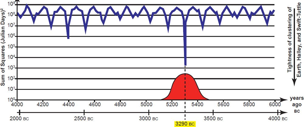
Fig. 1. This is Figure 233 directly reproduced from Brown (2014). The sum of the squares of the difference in time each year from calculated perihelion of either comet is plotted versus time. Notice that time increases to the left, with the most ancient time to the right.
Discussion
Brown went on to conduct two additional steps to determine some statistical significance of his result, but before discussing those, I need to address the question of how reliable Brown’s ephemerides are. Using Brown’s numbers, I was able to spot-check some of his entries in step two, and they appear to be correct. However, I used Brown’s technique with what I thought might be more reliable ephemerides, from which I got very different results. Additionally, instead of using a midsummer date each year, I used an approximation to January 1. The choice of date each year is not important—use of a different date each year will produce slightly different numerical values, but the times that the functions minimize will not significantly change. More importantly, I question Brown’s choice of “oldest known perihelion” and “oldest known period.” Brown used the earliest computed dates of perihelion passage of either comet from the two aforementioned papers, but that is not the same as the earliest truly known perihelion passages in the sense that they were observed. Chirikov and Vecheslavov (1989) noted that the earliest historical record that we have for Comet Halley is from 240 BC, and Yau, Yeomans, and Weissman (1994) similarly pointed out that the earliest historical record of Comet Swift-Tuttle was in 69 BC. Using computed epochs of Comet Halley more than a millennium prior to its first historical record and for Comet Swift-Tuttle more than a half millennium before its first historical record is an extrapolation. Therefore, I did my own computation using the earliest recorded perihelia (240 BC for Comet Halley and 69 BC for Comet Swift-Tuttle), which is a more objective definition of the earliest known perihelion for either comet.
There remains the question of which period to use for either comet. Brown chose to use the computed periods from step one at the earliest computed perihelion passage from the literature for either comet. Because Chirikov and Vecheslavov (1989) did not list periods at each perihelion passage for Comet Halley that they tabulated, this could be a legitimate choice. However, Yau, Yeomans, and Weissman (1994) did list a period at each perihelion passage. The period that they determined for Comet Swift-Tuttle at their computed 703 BC perihelion passage was 132.05 years, nearly three years less than the 129.33 year period that Brown used. It is inconsistent for Brown to use the epoch of Chirikov and Vecheslavov (1989) but not their period for that epoch. If Brown had used this alternate period with this epoch, he would have produced a very different result. Which period ought one to use? For the 22 computed perihelion passages for Comet Swift-Tuttle, Chirikov and Vecheslavov (1989) found periods between 127.37 years (AD 826) and 136.46 years (AD 1212), a range of more than nine years. Brown’s step one tabulated “true period” for Comet Swift-Tuttle lies between 124.00 years (AD 940) and 135.49 years (AD 1348), a range of more than 11 years. Similarly, Brown’s step one results for Comet Halley gives a minimum period of 67.68 years (1198 BC) and a maximum of 79.25 years (AD 530), a range of nearly a dozen years. One could use the average periods, 75.30 years for Comet Halley and 128.32 years for Comet Swift-Tuttle. Therefore, there is a tremendous range in ephemerides that one could use. Different ephemerides produce very different results, as I shall now demonstrate.
For my step two computation for Comet Halley, I decided to use the ephemeris consisting of the earliest known observed return in 240 BC and the average period computed in step one (75.297 years). For my step two computation for Comet Swift-Tuttle, I used the earliest known observed return in 69 BC, but, since Comet Swift-Tuttle has been observed on such few returns, I chose to use the step one computed period at the 69 BC epoch, 126.274 years. The period that Brown used for Comet Swift-Tuttle is slightly closer to the average period than the one that I used. However, the period that I used for Comet Halley is much closer to the average period than what Brown used. Using these alternate ephemerides for either comet, I did the identical step two computation that Brown did, but I got very different results, shown in Fig. 2. As with Brown’s plot, one can readily see the dips with the period of Comet Swift-Tuttle’s period modulated by the dips from Comet Halley’s period. There is no deep minimum at 3290 BC as with Brown’s plot, nor is there a more modest minimum near 2400 BC indicating when both comets might have come to perihelion just a few years apart. However, there is a noticeable minimum in the year 2349 BC, indicating that with the ephemerides that I used, both comets came to perihelion within a year of that date. Considering the uncertainty in the ephemerides this is remarkable, because this is the exact date that Ussher computed for the Flood. That is, using Brown’s model and methodology, one could just as well conclude that I have confirmed Ussher’s date for the Flood.
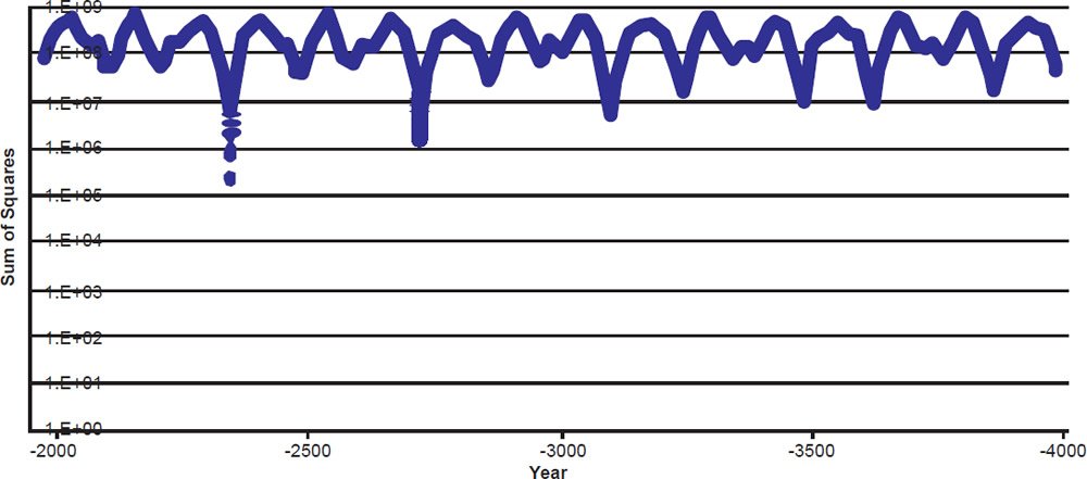
Fig. 2. Plot similar to that of Fig. 1, but computed with alternate ephemerides.
Now, I am not claiming that I have confirmed Ussher’s date of the Flood, for I reject Brown’s model for the origin of comets upon which my computation was based. Furthermore, given the great uncertainty in extrapolating the comet ephemerides so far into the past (discussed below), there are grave reservations about ability of dating the Flood using Brown’s approach. Finally, there is doubt that Ussher’s method of establishing chronology can produce such an exact date for the Flood. Ussher’s date for the Flood relies upon certain assumptions, such as the length of Israel’s sojourn in Egypt. A recent paper (Hardy and Carter 2014) reconsidered many of Ussher’s assumptions and concluded a likely range of dates for the Flood between 2600 BC—2300 BC (following the Masoretic text), with an absolute maximum range of 3386 BC—2256 BC (allowing for the LXX as well as the Masoretic text and a few other assumptions). Rather, I am illustrating the uncertainty in Brown’s methodology. The problem is that he has misused the information that he gleaned from the literature. The study of Comet Swift-Tuttle (Yau, Yeomans, and Weissman 1994) appears to have had several purposes, such as providing possible dates of visibility in the past with which we could correlate historical observations. However, extrapolating accurate dates of perihelion passages into the ancient past does not appear to be one of the purposes of that study. Indeed, that study stated,
Without constraints from early observations, a continuation of the integration backwards for any substantial length of time has relatively little value. For the present investigation, we have continued optimistically until the return of 703 BC. The close approach to Jupiter of 1.72 au on 323 BC April 10, and a subsequent close approach to the Earth of 0.247 au on 447 BC July 1, might have perturbed the motion of Comet Swift-Tuttle to such an extent that its orbit becomes unreliable beyond 447 BC. (Yau, Yeomans, and Weissman 1994, p. 314)
Brown chose to ignore this warning by treating the computed 703 BC perihelion passage as reliable, even though that date is two cycles past the last reliable computation. Likewise, Chirikov and Vecheslavov (1989) described the long-term motion of Comet Halley as chaotic. They noted that prior to 87 BC its motion was much less predictable than now. They also noted that near the end of their extrapolation the error was approximately five years. Again, Brown chose to ignore this warning in treating the earliest computed perihelion passage as reliable. His date for the Flood is nearly two millennia earlier than the earliest computed perihelion passage of Halley’s Comet than those tabulated by Chirikov and Vecheslavov. This is 27 cycles earlier. If the error in the computed times of perihelion was five years in the late second millennium BC, it easily could be decades late in the fourth millennium BC. For Comet Swift-Tuttle, Brown extrapolated 20 cycles earlier than his supposed “earliest known perihelion.” However, his extrapolation actually is 23 cycles earlier than the earliest historically known perihelion. Yau, Yeomans, and Weissman computed only 21 cycles into the past. With such gross extrapolations, computed times of perihelion passage of either comet in the fourth millennium BC could be off by decades, so any claims of a coincidence of perihelion passage of both comets then is unsupportable.
In his steps three and four, Brown conducted some sophisticated statistical analysis to assess errors and to gauge the probability that his conclusion was correct. In step three, Brown did a large number of random marches and concluded that only 0.6% of those random trials produced a clustering as tight as the one that he found. Brown alternately expressed this as having to search 333,333 years to find a clustering as tight as the one that he found. Of course, this simulation assumes that his ephemerides were correct, so this result is spurious if his ephemerides are not correct. In step four, Brown applied three different analyses to conclude that the error in the date of the coincidence of the two comets was about a century. That is, he has confidence that date of the Flood as determined by his method was 3290 BC, ± 100 years. For instance, Brown wrote:
Given that we are 99.4% confident that Halley and Swift-Tuttle were both near Earth in the same year, we will add the constraint to Figures A and B above that Halley made its 27th perihelion pass in the same year Swift-Tuttle made its 21st perihelion pass. (Brown 2014)
However, a century exceeds the orbital period of Comet Halley and comes close to the orbital period of Comet Swift-Tuttle. Allowing for a century variance in the computed date of the Flood, then the date could have coincided with the 26th or 28th perihelion passage of Comet Halley from his assumed initial epoch, not the 27th. This statistical analysis is meaningless. As I previously showed, to claim confidence in a calculation of perihelion passage for two comets in the same year in the fourth millennium BC is nonsense, and no amount of statistical analysis can improve that situation.
Conclusion
This was not Brown’s first attempt to astronomically establish the date of the Flood. A year earlier, Brown produced a similar calculation using Comet Halley and Comet Swift-Tuttle, but also three other periodic comets, 12P/Pons-Brooks, 13P/Olbers, and 23P/Brorsen-Metcalf (Brown 2013). Brown concluded the five comets were clustered in perihelion in 3346.5 BC, with an error of one year either way. Apparently, within a year of his earlier work, Brown realized that there were problems with his approach, and he modified it and deleted three of the comets from his later calculation. Also, he increased the error from one year to 100. The content of Brown’s website has been altered, so the earlier study is not available anymore.
I previously analyzed astronomical aspects of the hydroplate model (Faulkner 2013). Nearly a year after publication, I received correspondence from a hydroplate model supporter who challenged me on my charge that Brown had invoked an ad hoc explanation for why the deuterium content of the earth’s oceans and comets differed. This person told me that Brown had already answered this objection on his website. I replied that I had defined the eighth edition of Brown’s book (Brown 2008) as the standard by which I evaluated the hydroplate model, and that Brown’s explanation that this person referred to was absent from that book. My primary reason for insisting upon the latest printed version of the model was that the content of Brown’s website continually changes. It is impossible to make any up-to-date critique of such a voluminous and continually changing source, but a printed copy that is readily available after publication is a fixed standard. The rapidly changing approach that Brown has regarding his claim to astronomically date the year of the Flood demonstrates the wisdom of that standard. Here I made an exception to my general rule not to discuss Brown’s online work. I expect that Brown’s computation of the date of the Flood to further change, perhaps in response to this critique.
Consider again Fig. 1, the plot of Brown’s sum of squared differences. As I previously noted (but Brown did not), there is a modest dip near 2400 BC. This corresponds to a time, according to Brown’s adopted ephemerides, that both comets came to perihelion less than three years apart. Comet Swift-Tuttle came to perihelion on December 26, 2385 BC, followed by Comet Halley at perihelion on September 10, 2382 BC. Both Comet Halley and Comet Swift-Tuttle have had observed period changes from one apparition to the next that exceed the difference between these two dates,3 so it is quite plausible to propose that these two comets actually came to perihelion at the same time around 2382 BC—2385 BC. This is within a half century of the Ussher chronology. Hence, by Brown’s own methodology, one could make the case that this is the astronomically determined date of the Flood. Recall that with alternate ephemerides, I found a date that agrees with the Ussher date precisely. One could produce numerous other possible Flood dates by using only slightly different ephemerides. Obviously, all of these dates cannot be correct, and probably none of them are. This illustrates the futility of Brown’s approach. It is doubtful that this technique can be used to date the Flood. This also illustrates the danger of blurring the distinction between observational/experimental science and historical or origin science. Evolutionary scientists frequently do this, so we creationists need to be cautious in our approach as well when discussing past events. Reliable historical documents, such as the Bible, are much more reliable than an approach using multiple assumptions and extrapolations.
References
Brown, W. 2008. In the beginning: Compelling evidence for Creation and the Flood. Center for Scientific Creation, Phoenix, Arizona.
Brown, W. 2013. http://www.creationscience.com/onlinebook/FAQ212.html. Accessed June 7, 2013.
Brown, W. 2014. http://www.creationscience.com/onlinebook/TechnicalNotes2.html. Accessed August 15, 2014.
Brown, W. 2015. http://www.creationscience.com/onlinebook/FAQ213.html. Accessed January 12, 2015.
Chirikov R. V., and V. V. Vecheslavov. 1989. Chaotic dynamics of comet Halley. Astronomy and Astrophysics 221:146–154.
Dybczynski, P. A. 2001. Dynamical history of the observed long-period comets. Astronomy and Astrophysics 375, no. 2:643–650.
Faulkner, D. R. 2013. An analysis of astronomical aspects of the hydroplate theory. Creation Research Society Quarterly 49, no. 3:197–210.
Hardy, C., and R. Carter. 2014. The biblical minimum and maximum age of the Flood. Journal of Creation 28, no. 2:89–96.
Yau, K., D. Yeomans, and P. Weissman. 1994. The past and future motion of Comet P/Swift-Tuttle. Monthly Notices of the Royal Astronomical Society 266:305–316.
Yeomans, D. 1997. http://www2.jpl.nasa.gov/comet/ephemjpl8.html.


