Revisiting an Iconic Argument for Milankovitch Climate Forcing: Should the “Pacemaker of the Ice Ages” Paper Be Retracted? Part 2

Introduction

The Milankovitch hypothesis is the dominant explanation for the 50 or so supposed Pleistocene ice ages (Walker and Lowe 2007). It was proposed by J. A. Adhémar in 1842, modified by James Croll in the mid to late 1800s, and was later quantitatively refined by Serbian geophysicist Milutin Milanković (Imbrie 1982; Milanković 1941). Summaries of the hypothesis are provided elsewhere (Hebert 2014, 2015, 2016).

Despite many difficulties (Cronin 2010, 130–139; Oard 2007), the hypothesis is generally thought to have been elevated to the status of theory by an iconic 1976 paper in Science entitled “Variations in the Earth’s Orbit: Pacemaker of the Ice Ages” (Hays, Imbrie, and Shackleton 1976, hereafter referred to as Pacemaker). Hays, Imbrie, and Shackleton performed spectral analyses on three variables of presumed climatic significance within the two Indian Ocean sediment cores RC11-120 and E49-18. Spectral analyses of oxygen isotope ratios of the planktonic foraminiferal species Globigerina bulloides, the relative abundance of the radiolarian species Cycladophora davisiana, and (southern hemisphere) summer sea surface temperatures (SST), also inferred from radiolarian data, revealed spectral peaks corresponding to periods of approximately 100, 41, and 23 ka. These periods also correspond to those of dominant cycles in the earth’s orbital motions. Hence, the Milankovitch hypothesis is widely seen as having been confirmed by the Pacemaker paper.

Fourier Analysis

Part I of this series (Hebert 2016) presented an overview of a number of serious problems with the Pacemaker paper. To truly understand Pacemaker, however, it is necessary to also understand the Blackman-Tukey (B-T) method (Blackman and Tukey 1958) of spectral analysis. Readers already familiar with this method may choose to skip ahead to the section entitled “Replication of Results: RC11-120.”

Understanding the Blackman-Tukey method in turn requires a brief discussion of Fourier analysis.

A continuous function g(t) may be represented as the sum of an infinite number of waves of varying frequencies and frequency-dependent (and possibly complex) amplitudes A(f):

Some mathematical manipulation results in an expression for the frequency-dependent amplitude A(f). This amplitude is known as the Fourier transform (FT) of g(t):

The frequency-dependent spectral power density, which we denote as Γ(f), is proportional to the modulus squared of the Fourier transform:

The constant C_N is a normalization constant, which I discuss in more detail later. For now, the key point is that waves characterized by larger amplitudes make a larger contribution to the signal g(t). If one makes a plot of Γ(f) versus frequency f, pronounced peaks will occur at the frequencies of the waves making very large contributions to the signal.

If one replaces f by –f in Eqs. (2) and (3), one may show that

One can make use of this fact to define a one-sided (defined for non-negative frequencies only) spectral power density such that

The above equations assume that g(t) is a continuous function, but in analyzing seafloor sediment data, one actually only has discrete values of a given variable to analyze. For this reason, researchers often use discrete versions of Fourier transforms (DFTs) in order to analyze paleoclimatological data. For n discrete values of a variable g(t) = {g(t₀), g(t₁), . . . g(t_n-1)} that are equally spaced in time, the DFT may be written as:

One may wonder why each term in the sum of Eq. 6 does not contain a Δt, by analogy with Eq. 2. The discrete Fourier transform is usually defined in such a way that the constant time increment Δt is pulled out of the summation (Press et al. 2007, 607).

A plot of spectral power versus frequency obtained in this manner is called a periodogram (Muller and MacDonald 2000, 55).When using a DFT to calculate a periodogram, one often calculates power values for n/2 independent frequencies. This makes sense when one considers the periodogram’s information content. The periodogram contains no information about the phases of the waves comprising the signal, only their frequencies. Hence, the periodogram contains only half the information content of the original n data points (Muller and MacDonald 2000, 49–50). However, practitioners often pad the end of the sequence of n data points with a string of zeros so as to effectively increase the number of data points and hence the periodogram’s frequency resolution (Muller and MacDonald 2000, 60–61). However, such padding complicates assessment of the significance of results (Weedon 2003, 65).

If the mean of the signal is non-zero, then Γ(f = 0) will be very large compared to the powers at non-zero frequencies and will tend to dominate the power spectrum. Hence, the data are usually detrended prior to performing a spectral analysis. This can be done by subtracting the mean of the data from each data point or by performing a linear regression on the data (any trend in seafloor sediment data is usually very slight) and then replacing the data by the residuals from the linear regression (Hays, Imbrie, and Shackleton 1976, 1125, 1132; Muller and MacDonald 2000, 50).

A particularly fast, efficient way to perform a DFT is via a “Fast Fourier Transform,” or FFT. For those unfamiliar with DFTs and FFTs, detailed discussions are provided in (Press et al. 2007, 608–639). However, because FFTs can be somewhat confusing to the uninitiated (Muller and MacDonald 2000, 51) due to their use of negative frequencies, this paper will not discuss them any further. Given the speed with which modern computers can perform calculations and the relatively small size of the data sets used in the Pacemaker paper, little is gained by using a FFT to perform the calculations.

Normalization of the DFT

As stated earlier, the squared moduli of the frequency-dependent amplitudes indicate the relative contribution that a wave of particular frequency is making to the signal. More precisely, we can define the variance (square of the standard deviation) of the finite, real, detrended, discrete data set as

I then impose the following normalization condition:

where C_N is a normalization constant. I discuss this normalization condition in more detail in the following sections.

Weaknesses of the DFT

A DFT requires all the data points to be evenly spaced in time. This is problematic for a number of reasons. First, one rarely encounters evenly spaced times in analyses of seafloor sediment data. Even if measurements are made within a core at equally spaced distance intervals, the times assigned to these distances will almost never be evenly spaced. Obtaining evenly spaced times thus requires the use of an interpolation process. This introduces error, since the spectral analysis is then performed, not on the original data, but on interpolations from that data. Interpolation tends to enhance the power of low frequency components at the expense of the higher frequencies (Schulz and Mudelsee 2002, 421). Unfortunately, most spectral analysis methods require equally spaced data, including the B-T method used in Pacemaker.

Second, statisticians would say that the DFT estimator of spectral power has a large variance, and this variance does not decrease with increasing sample size; i.e., estimates of spectral power are erratic (Jenkins and Watts 1968, 211–213). Hence, the estimate for the power spectrum that one obtains is not necessarily equal to the true power spectrum. One would like an estimator of a given quantity to have both low variance and to be unbiased (i.e., estimates for a given parameter are not systematically too high or too low). Unfortunately, these two criteria can be difficult to balance. The B-T method is an attempt to decrease the variance of the spectral estimator while minimizing bias as much as possible.

Third, the use of data points that are spaced evenly in time introduces a problem called aliasing: waves of one frequency may be mistaken for waves of another frequency. In order to discuss aliasing, we must introduce a quantity called the Nyquist frequency, the highest frequency that can appear in a DFT (Muller and MacDonald 2000, 50).

The Nyquist Frequency

As a practical matter, one cannot, nor would one wish to, perform calculations using an infinite range of frequencies. What therefore is the appropriate upper frequency limit on Eq. (8)? The problem of aliasing suggests an answer to that question.

The time interval Δt separating equally spaced measurements is called the sampling interval, and the reciprocal of the sampling interval is called the sampling frequency, f_s. Fig. 1 (after Blackman and Tukey’s Fig. 7, 31) illustrates how a set of discrete data points (open black circles) collected at a constant sampling interval of 0.2 s could be caused by either a wave of frequency f = 1 Hz or another wave of frequency f = 4 Hz. This phenomenon is called aliasing.

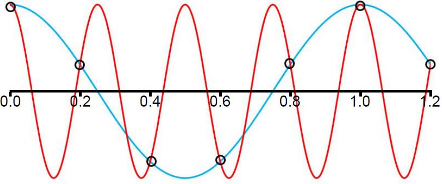
Fig. 1. If the open black circles represent actual sampled data points (with a sampling interval of 0.2 s), then these data points could be the result of a wave of frequency f = 1 cycle/second (blue line) or a wave of frequency f = 4 cycles/second (red line).

A sampling frequency of 2f is the bare minimum needed in order to detect a wave of frequency f. Hence the wave must be sampled at least twice during a wave cycle, such as at the two times per cycle at which the wave is at its minimum and maximum values. We call the highest detectable frequency in a signal (Jenkins and Watts 1968, 211) the Nyquist frequency, indicated by the symbol f_Nyq. Hence the sampling frequency will be twice the Nyquist frequency. Or equivalently, the Nyquist frequency will be half the sampling frequency:

Since the DC component of the signal has been removed by detrending, the smallest frequency of interest, f_min, is 1/T, where T is the total length of time for which data have been collected.

Because of aliasing, frequencies higher than the Nyquist frequency can make contributions to the calculated spectral power spectrum. For this and other reasons, our calculated power spectrum is at best an approximation to the true power spectrum. As a practical matter, however, aliasing is not much of a problem in dealing with seafloor sediment data, because processes that blur the signal (such as bioturbation) tend to reduce aliasing effects (Muller and MacDonald 2000, 62).

We can now further clarify the proper normalization of the DFT. Because the spectral power values are independent of one another, one cannot really infer anything about power values at frequencies other than the discrete frequencies of the periodogram. Some analysts emphasize this point by using separated vertical lines or dots rather than a smooth curve to indicate spectral power obtained by a DFT (Weedon 2003, 68). Since the spectrum is undefined at other in between frequencies, normalization may be achieved by demanding that the simple sum of each of the discrete values of P(f_i) = 2Γ(f_i) add up to the total variance of the original signal:

In Eq. (10), the sums are over n/2 non-negative, equally spaced frequencies ranging from f_min = 1/T to f_max = f_Nyq.

DFT Demonstration

Fig. 2 illustrates a signal formed by superposing two different waves, one of frequency 1 Hz and the other of frequency 4 Hz. The 1 Hz wave has an amplitude three times greater than that of the 4 Hz wave. In this case, the time ranged from 0.0 to 10.35 s, with Δt = 0.05 s. The total variance of this signal, in arbitrary units, is 5.0225. Fig. 3 shows the normalized power spectrum for this signal. Although the Nyquist frequency is indeed 10.0 Hz, as one would expect from Eq. (9), I have only plotted spectral power values up to 5.0 Hz, so that the details in the interesting part of the plot may be seen more easily (the rest of the power spectrum is flat). The spectrum is characterized by two dominant peaks located very close to the frequencies of the two waves which comprised the signal. Because none of the discrete frequencies of the transform corresponded to exactly 1 or 4 Hz, these peaks are shifted slightly from the expected frequencies. These small discrepancies result in resolution bias (the picket fence effect): from Eq. (3), one might expect the height of the 1 Hz peak to be exactly nine times greater than the height of the 4 Hz peak. However, this is not the case, due to resolution bias: because the true frequencies of the two waves lie between the specified frequencies of the DFT, the peaks tend to be too low and the troughs tend to be too high (see http://azimadli.com/vibman/thepicketfenceeffect.htm for an illustration). However, in analysis of seafloor sediment data, one generally is not concerned with the precise values of the spectral powers, so the picket fence effect is not of great concern.

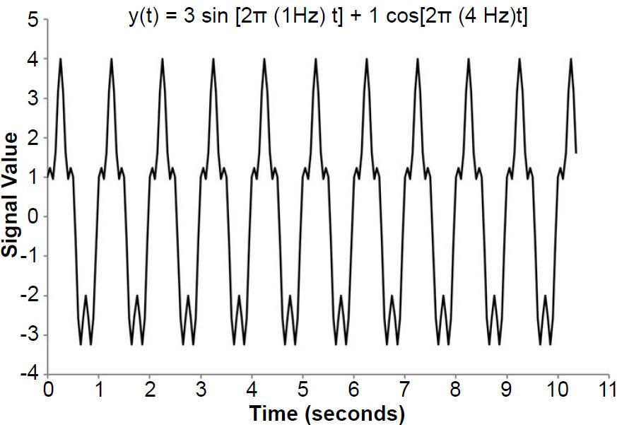
Fig. 2. Waveform generated by superposing a 1 Hz sine wave (amplitude of 3) with a 4 Hz cosine wave (amplitude of 1).

---

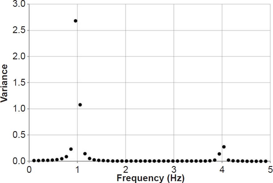
Fig. 3. Power spectrum generated from the waveform in Fig. 2 using a discrete Fourier transform.

Spectral Leakage

However, another phenomenon, called spectral leakage, can be more problematic in analysis of seafloor sediment data. Some of the spectral power expected at a particular frequency can be leaked to adjacent frequencies. Little spectral leakage is apparent in Fig. 3, but it is generally more noticeable, with ripples or sidelobes on either side of a true spectral peak.

Spectral leakage results from the fact that we are obtaining the Fourier transform, not of the original signal g(t) per se, which is infinite in extent, but the original signal multiplied by a rectangular box function w(t), defined by

Suppose that the original signal is a pure sinusoid of frequency f₀. To simplify the notation somewhat, we express this sinusoid in terms of the angular frequency ω₀ = 2πf₀:

Because we measured g(t) only for a finite time of length T, the function whose Fourier transform we obtained was actually g(t)w(t). Using the form of the Fourier transform expressed in terms of angular frequency ω (Arfken and Weber 2005, 931), the Fourier transform of the product becomes

Integrating Eq. (13) yields the sinc function:

Hence the (unnormalized) apparent spectral power at an angular frequency ω will be

Normalization of the above result was achieved by numerically integrating Eq. (15) over a range of angular frequencies beyond which the value of P_app(ω) could safely be taken to be essentially zero, i.e., from ω = −20.0 rads/s to ω = +20.0 rads/s, in steps of 0.05 rads/s. This integration yielded a value of 9.968 s, which agrees well with the analytical result: integration of Eq. (15) from negative to positive infinity yields a result of T, or 10.0 s. This result was then equated to the analytically obtained variance of g(t) over the interval t = −T/2 to t = +T/2, i.e., the average value of the square of g(t) from −5.0 s to +5.0 s. Fig. 4 is a graph of the resulting normalized P_app(ω) for ω₀ = 2.0 rads/s and T = 10.0 s. In the absence of windowing by the block function, one would expect the power spectrum to consist of a single sharp spike centered on 2.0 rads/s. But because we took the Fourier transform of a sinusoid of finite extent, rather than the original sinusoid of infinite extent, the spectral power was leaked to other frequencies, with the worst leakage occurring for frequencies near ω₀. This leakage is characterized by ripples, or sidelobes, to the left and right of the main peak. If a second smaller peak is located near this main peak, the sidelobes surrounding the first peak could potentially bias power estimates for the smaller peak (Muller and MacDonald 2000, 71). This is especially true for high-frequency signals of low amplitude (Weedon 2003, 63). Hence it is often desirable to reduce spectral leakage by use of a taper or window.

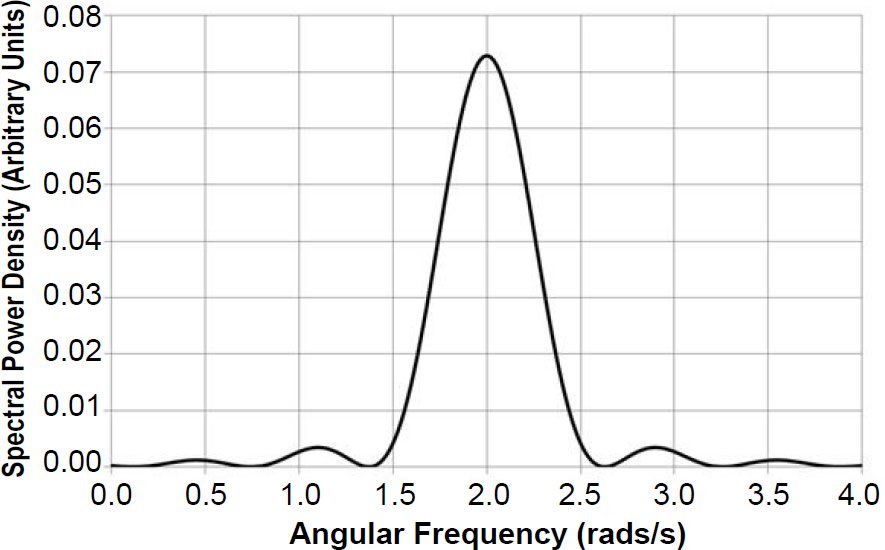
Fig. 4. The power spectrum of a simple sinusoidal wave of angular frequency ω₀ = 2.0 rads/s demonstrates the phenomenon of spectral leakage.

Tapering

An accepted method for reducing spectral leakage is to use a smooth window (or taper) other than the non-smooth block function, preferably a taper that smoothly approaches 1 near the center of the observed time and 0 at the edges of this timeframe. As an example, consider a cosine window function defined by

This window is defined such that it is equal to 1 at t = 0 and equal to 0 at t = −T/2 and t = T/2 (as well as equal to 0 for values of t such that |t| > T/2). Our original signal g(t) is again a pure sinusoid of angular frequency ω₀. The Fourier transform of g(t) w(t) becomes

Making use of the Euler identity and the symmetry properties of the integral, this reduces to

Eq. (18) may be simplified with the following trigonometric identity (Spiegel 1994, 17):

Substitution and integration yields an expression for the Fourier transform that is the sum of two sinc functions:

This can be further simplified to

Applying the same normalization procedure used earlier yields the power spectrum shown in Fig. 5. The leakage in Fig. 5 has been reduced, but at the cost of lower resolution: the peak at ω₀ = 2.0 rads/s has been broadened, with an accompanying decrease in the amplitude of the central peak.

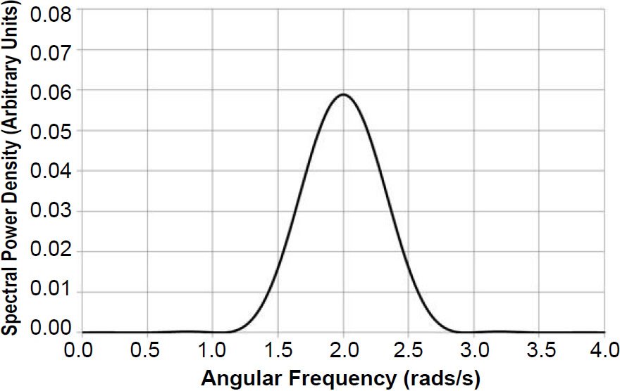
Fig. 5. Application of a cosine taper reduces the leakage but at the cost of a broadened spectral peak of lower amplitude.

There are a number of different tapers frequently used in spectral analysis, and these are usually defined to be simple, slowly-varying functions that go to zero near the edges (Muller and MacDonald 2000, 70). The mathematical forms of a number of well-known tapers were obtained more by trial and error than any particular mathematical theory (Blackman and Tukey 1958, 14). When using the B-T method, the width of the taper is chosen such that it has a minimum value, not necessarily at t = T, but for a pre-determined time value (lag) τ that can be less than T. Since the data points are equally spaced in time, the lags may be expressed in terms of integer multiples of the time increment Δt. In other words, the lag is given by τ = lΔt, where l is an integer. The maximum lag value is given by τ_max = mΔt, where m is the integer value corresponding to the maximum lag. The Pacemaker authors used what is known as a Hamming taper (Hays, Imbrie, and Shackleton 1976, 1125; Muller and MacDonald 2000, 70), defined as:

However, it is not the kind of taper, but the width of the taper that is of greatest importance (Jenkins and Watts 1968, 273). This width influences a quantity called bandwidth (discussed below).

The above version of the Hamming taper is designed to have minima when l equals 0 or m and a maximum value when l = m/2. For a B-T analysis of data values collected at times ranging from t = 0 to t = T, the appropriate version of the Hamming taper is given by

In this version of the Hamming window, the window will have a value of 1 when l = 0 and a minimum value when l = m. Hence g(t = 0) is unaffected by the Hamming window, but the window effectively reduces g(t = mΔt) to only 8% of its original value.

Autocovariance

A fair test of the Milankovitch hypothesis should take into account uncertainty in age estimates. The Pacemaker authors assumed constant sedimentation rates for the two cores which they analyzed (their SIMPLEX age models). After obtaining results generally consistent with Milankovitch expectations, they then experimented with more complicated age models. Of course, even uniformitarians do not believe that sedimentation rates have been perfectly constant for hundreds of thousands of years, so such a test should make allowances for possible changes in sedimentation rate. The B-T method is a good choice for paleoclimate work in which the timescale is uncertain (Tukey himself is said to have recommended it), as it blurs the power spectrum (Muller and MacDonald 2000, 16, 63–66). It makes use of a theorem that states that the Fourier transform of a function’s autocovariance is equal to that function’s spectral power density. Blackman and Tukey (1958, 5) define the autocovariance of a real function g(t) (having zero mean) for a given lag τ to be:

Eq. (24) is actually the average value (Thomas and Finney 1988, 341) of g(t)g(t + τ). One may demonstrate that the autocovariance is an even function (a fact that will become important shortly) by first making the substitution τ → −τ and then the substitution t → t + τ. We now express autocovariance in a one-sided form:

Derivation of the B-T Method

A consequence of the Wiener-Khintchin theorem (Blackman and Tukey 1958, 8; Khintchin 1934; Wiener 1930) is the fact that the Fourier transform of g(t)’s autocovariance is equal to g(t)’s spectral power density:

Making use of symmetry, the Euler identity, and the fact that the autocovariance function is even yields

which implies that P(f) is

In actual practice, our data sets will be of finite length. Expressing Eq. (25) in a discrete form for a finite number of n data points gives

The subscript S in Eq. (29) indicates that this is now a sample autocovariance. Suppose we have a set of n data points, and we indicate each data point with an index i ranging from 0 to n−1. The sample autocovariance will be defined for lags ranging from l = 0 up to some maximum lag of our choosing that we designate by l = m. The maximum lag we choose will in turn determine the number of terms in the sum of Eq. (29). As a simple example, suppose that we have n = 9 data points (Fig. 6), with the first data point

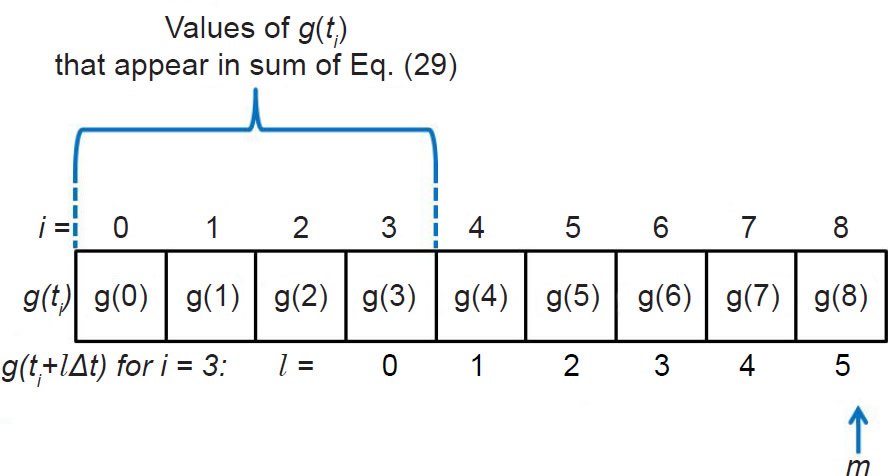
Fig. 6. The choice for the maximum lag m will determine the number of terms in the sum of Eq. (29).

designated by i = 0 and the last data point by i = 8. Let us also suppose that we choose our maximum lag to correspond to m = 5. In order to do our calculation for m = 5, we must be able to multiply every g(t_i) in our sum by a corresponding g(t_i + 5Δt) that is five elements to its right, and this must also be true for the very last element in our sum. Hence, we must count backwards from 5 to 0 from our very last data point (corresponding to i = 8) to determine which data point will be last in the sum. If we do so, we see that this last element corresponds to i = 3.

This implies that for l = m = 5, there will be four terms in the sum, as we would expect from Fig. 6. Likewise the denominator in the fraction will be 4Δt. Hence the right side of Eq. (29) is actually the average value of g(t_i)g(t_i + lΔt) for the four g(t_i) values in the sum, which is consistent with our understanding of Eqs. (24) and (25).

Now consider two extreme cases. Suppose that we calculate only one autocovariance value, that corresponding to l = m = 0. In this case, our autocovariance is simply the average of g(t_i)² calculated with nine terms, the maximum possible.

On the other hand, suppose we calculate autocovariance values for the maximum possible number of lags (nine). This maximum lag will correspond to m = l = 8. But in order to do this, our average can be calculated with only one term, that corresponding to i = 0.

Blurring of the Power Spectrum

The previous discussion and Eq. (29) give insight into why the B-T method is useful. As just noted, the larger the maximum lag τ_max = mΔt, the fewer the number of terms that will appear in the sum. But a small number of terms in the sum implies a poor estimate for the average of g(t)g(t + τ). This implies that our estimator for spectral power will be subject to high variance. Increasing the number of terms in the sum improves the estimate of the average (and hence of spectral power). Hence, this is one reason the B-T method is useful: it is a more stable estimator of spectral power than a DFT, at least for relatively small lags.

The B-T method blurs the power spectrum, resulting in a decrease in resolution. However, some degree of blurring is good, as drifts in timescale caused by small changes in sedimentation rate can cause spurious peaks to appear in the power spectrum. The B-T method causes these sidelobes to be absorbed into the real peak, giving a better estimate of spectral power (Muller and MacDonald 2000, 65).

The degree of blurring (assuming no windowing) depends on the number of terms that appear in the sum of Eq. (29). The proof is most easily performed using Eqs. (25) (for a finite value of T) and (26). If only 1/3 the total length of time T is used to calculate the integral in the expression for the sample autocovariance, then continuous lag values may be calculated for the remaining 2/3 of the total time. Muller and MacDonald (2000, 64–65) show that this implies that the resolution will be about 3/2 = 1.5 times poorer than would be the case for a simple Fourier transform. However, the use of a smooth taper decreases resolution still further (Muller and MacDonald 2000, 55).

Important Formulae

Experts (that is, Jenkins and Watts 1968, 174–180) recommend using the so-called biased estimator of the sample autocovariance function:

Taking the Fourier transform of the unbiased expression for autocovariance found in Eq. (29) would give greatest weight to the autocovariance values calculated with the smallest number of terms. Such an estimator of spectral power would be subject to a very high variance (Jenkins and Watts 1968, 179; Wunsch 2010, 67–68). Hence the biased expression for the sample autocovariance is preferred.

Furthermore, multiplying Eq. (30) by a taper (such as the Hamming taper) gives still greater weight to autocovariances for smaller lag values, which are calculated with a larger number of terms in the sum. This helps improve still further the estimate of spectral power.

Fig. 7 shows sample autocovariance values for m = 40 (untapered, and tapered with a Hamming window) calculated using my reconstructed δ¹⁸O values from the RC11-120 sediment core (Hebert 2016), after detrending and interpolation (with Δt = 3 ka).

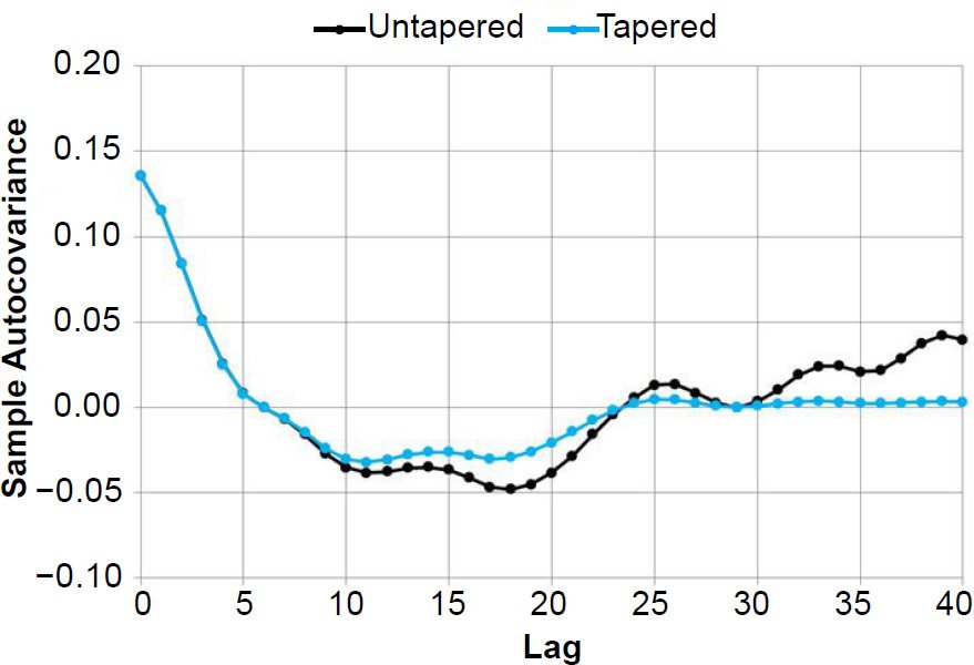
Figure. 7. Untapered and tapered (using a Hamming window) sample autocovariance values calculated for reconstructed δ¹⁸O values in the RC11-120 sediment core, with m = 40 (the same value used in the Pacemaker paper).

Remembering that τ = lΔt and multiplying A_S(τ) by a taper to obtain the tapered sample autocovariance A_ST (τ), we may express Eq. (28) in a discrete form to obtain the B-T estimate of spectral power at a frequency f:

One may wonder why the summation goes to l = m−1 rather than l = m. Because τ = 0 corresponds to l = 0, the index l corresponds to the left-hand side of each time increment Δt, not the right-hand side. If the summation went to l = m, then the sum would include a small contribution from the part of the sample autocorrelation function that is just a little to the right of τ = mΔt, even though we intend to truncate the sample autocorrelation at precisely τ = mΔt (see Jenkins and Watts 1968, 259–260).

Eqs. (30) and (31) allow us to calculate the spectral density function for a set of evenly spaced data points. Note that the l = 0 term makes a large non-zero contribution to the sum, which causes all frequencies to exhibit significant noticeable background power, which is not the result one obtains from using a DFT. This may be the reason that some authors prefer to give only half as much weight to the l = 0 term (i.e., see Jenkins and Watts 1968, 259):

Now that we have explained the fundamentals of the B-T method, we need to answer the question, what is the appropriate value of m to use for a particular analysis? In order to answer that question, we must briefly discuss a quantity called bandwidth.

Bandwidth

Our discussion of tapers or windows so far has only involved time domain expressions for these windows. As noted before, time is a function of lag, so these windows are sometimes expressed in terms of the lag value l and are called lag windows w(l). We denote as W(f) the spectral window, which is the Fourier transform (Jenkins and Watts 1968, 245) of w(l). In order to obtain a good estimate of a spectral peak, the width of the narrowest important feature in the spectrum should be roughly the same size as the width of the spectral window W(f) (Jenkins and Watts 1968, 256, 279). Of course, what is considered an important feature by one person may not be considered important by another. Hence, there is a subjective element in the method, and caution must be exercised when using it (Jenkins and Watts 1968, 281–282; Weedon 2003, 85).

This in turn raises the question of how one determines the width of a spectral window W(f). This width is defined by a quantity called bandwidth or equivalent bandwidth. Bandwidth, denoted by the letter b, is a measure of the frequency resolution of the spectral density estimate (Buttkus 2000, 192). A smaller bandwidth means greater frequency resolution, and vice versa. We denote with the letter h the width of a rectangular bandpass spectral window W_rec(f) which is defined in such a way that it is symmetric about f = 0. Thus, the bandwidth b of this rectangular window is equal to h. The bandwidth (or equivalent bandwidth) for a non-rectangular spectral window is the width of a rectangular window that will cause the spectral estimator to have the same variance as the estimator calculated with the non-rectangular window. Such discussions are found in many textbooks (Buttkus 2000, 196–197; Jenkins and Watts 1968, 255–257). Following this derivation, one may show that the reciprocal of the bandwidth b is the integral I of the square of the window function over all possible lag or frequency values:

The last equality in Eq. (33) is Parseval’s theorem. Because the windows are symmetric about f = 0 and l = 0, the Hamming window may be expressed as

One can use Eqs. (33) and (34) to verify that the bandwidth of the Hamming taper is given by (see Hays, Imbrie, and Shackleton 1976, 1132, their reference 57):

The uncertainty in the frequency of a peak may be taken to be plus or minus half the bandwidth (Weedon 2003, 59).

Blackman and Tukey argued that m should be restricted to a small fraction of the total number of data points (Blackman and Tukey 1958, 11), as do many other experts. However, if one takes seriously the requirement that b be on the order of the width of the smallest important feature in the power spectrum, then a larger value of m may be necessary in order to meet this requirement. Hence Eq. (35) gives us an indication of the approximate value of m that should be used for the spectral analysis. Since the bandwidth should be comparable to the width of the smallest important feature in the spectrum, m should be large enough to ensure that this will be the case, but preferably no larger, since still higher values of m will further decrease the stability of our B-T spectral density estimator.

How Many Frequency Bands?

There is no hard and fast connection between the number of frequency bands of width Δf and the maximum number of lags m (Jenkins and Watts 1968, 260). The Pacemaker authors set the number of frequency bands to m + 1 (Hays, Imbrie, and Shackleton 1976, 1132, their reference 57). Although one normally associates a frequency band with a range of frequencies (i.e., a value of Δf), I am assuming that by bands the Pacemaker authors actually meant the number of discrete frequency values used in their calculations. However, this is a small detail which will not greatly affect the final results. Jenkins and Watts (1968, 260) recommend using a frequency spacing that is 2–3 times smaller than this in order to reveal more detail in the power spectrum. Thus our final normalization condition for the B-T estimate of spectral power is

where C_N is a normalization constant.

Background Noise

Before one can discuss the possible statistical significance of results obtained in a spectrum analysis, one has to first determine the level of background noise. Seafloor sediment spectra are often characterized by red noise (Gilman, Fuglister, and Mitchell 1963). A power spectrum exhibiting red noise behavior can result from a time series generated by a discrete AR-1, or first-order autoregressive random process (Schulz and Mudelsee 2002). For both evenly and unevenly spaced data sets, it is possible to fit red noise models to the data (Mann and Lees 1996; Meyers 2012; Mudelsee 2002; Schulz and Mudelsee 2002).

A power spectrum exhibiting red noise is marked by a decrease of spectral amplitude with increasing frequency, with the rate of decrease greatest for lower frequencies. This is in contrast to a spectrum of approximately constant spectral amplitude as a function of frequency (white noise).

The Pacemaker authors obtained their estimate of spectral power of the background noise by producing a very smooth power spectrum. This smoothed power spectrum is called the null continuum because the null hypothesis is the default assumption that visible spectral peaks are not statistically distinguishable from the background spectral power. Only if the peaks are sufficiently pronounced is the null hypothesis disproven (we discuss this in more detail in the next section). Although the smoothed spectra produced by this method will often exhibit red noise characteristics (as is often the case with paleoclimatological data sets), this method makes no explicit assumptions about the random process generating the null continuum. The smooth background is obtained simply by setting m to an integer value that is a small fraction of the number of data points n. The following statement in a set of classroom notes describes this technique (Meko 2015, 9):

Another approach to a null continuum is empirically based and does not attempt to assign any particular theoretical generating model as a null hypothesis (Bloomfield 2000). This approach uses a greatly smoothed version of the raw periodogram as the null hypothesis. . . . The estimation of a null continuum by smoothing the periodogram relies on subjective judgement [sic] and trial-and-error. In particular the null continuum should follow just the smooth underlying shape of the distribution of variance over frequency. If smoothed insufficiently, the null continuum will bulge at the important peaks in the spectrum. This would clearly be undesirable as the test of significance of the peak is that it is different from the null continuum.

This process is demonstrated in Fig. 8, as power spectra for the detrended and interpolated RC11-120 δ¹⁸O values are calculated for values of m equal to 0, 2, 4, 6, 8, and 9. To be consistent with the methodology used in the Pacemaker paper, for all six estimates of the null continuum, the power spectra have been normalized so that the sum of the variances at all frequencies equals unity, or 100%. The higher frequency ripples for some values of m occasionally resulted in slightly negative spectral powers at high frequencies: these negative spectral powers were truncated and set equal to 0.0001 prior to normalization. A small positive number was chosen rather than zero in anticipation of the fact that semi-log plots of spectral power would eventually be needed. The number of frequencies was m + 1, as in the Pacemaker paper. Note that the background curve obtained by setting m = 0 (the smallest possible value of m) is extremely stable but very biased—a flat line. As m is gradually increased, the bias decreases, with the smoothed spectral power estimates near f = 0 becoming much more consistent (~10–12%). As noted earlier, some of the null continua exhibit oscillatory behavior at higher frequencies. One would presumably not expect a background spectrum to do this, so ideally one would like to choose a value of m that minimizes or eliminates this oscillatory behavior.

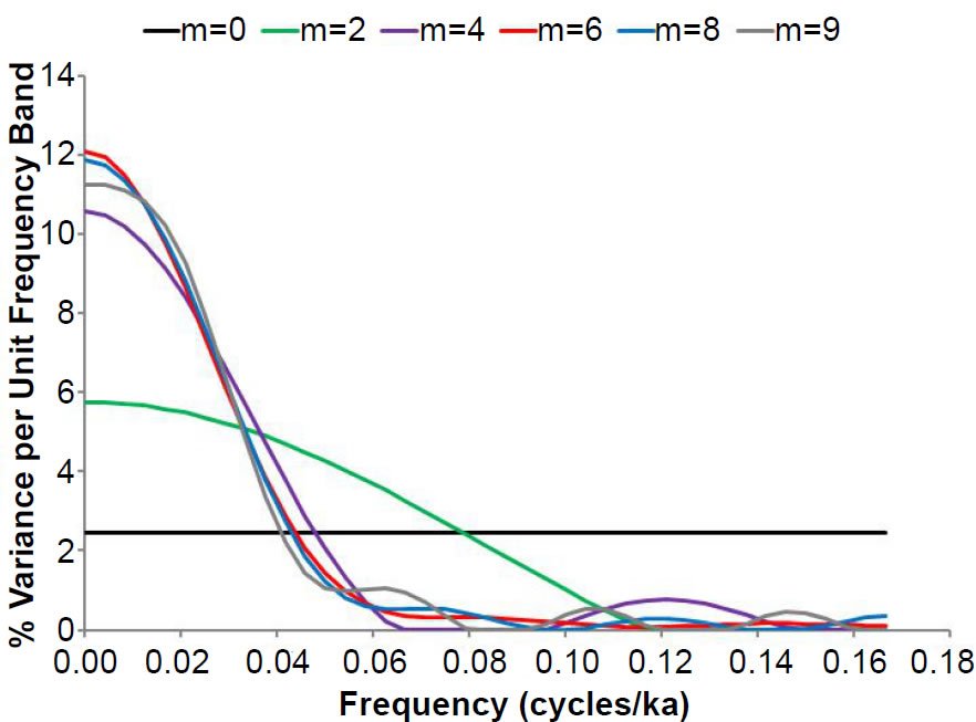
Fig. 8. Process used to determine the null continua for the Blackman-Tukey method. Power spectra are calculated for larger and larger values of m for oxygen isotope values in the RC11-120 core. Higher values of m decrease the bias, but at the cost of increasing instability of the power spectrum estimator.

Jenkins and Watts (1968, 263–272) recommended that one obtain the background spectrum by starting with very small value values of m, and increasing those values until still higher values of m do not appreciably decrease the bias. Following the lead of the Pacemaker authors, I will use just a single value of m to obtain the null continua for all three variables. In the δ¹⁸O case, a value of m = 6 or m = 7 (the two curves are practically indistinguishable) seems to give the best estimate of the null continuum spectrum: power decreases continuously with increasing frequency, with a greater rate of decrease at low frequencies, and the oscillatory behavior at higher frequencies has been significantly damped. Hence, the null continuum exhibits behavior that roughly approximates that of red noise, as one might expect from a seafloor sediment data set. The SST null continuum also exhibited approximate red noise behavior, with a value of m = 4 yielding the best result, although m values of 5–7 were also acceptable. If one attempts to make the null continuum for % C. davisiana follow the smooth underlying shape of the power spectrum, as suggested by Meko (2015), then a value of m = 9 is probably the best choice, but m values of 6, 7, and 8 also yielded similarly shaped null continua. However, such a null continuum would be noticeably different from a red noise spectrum, with a pronounced hump around f = 0.025 cycles/ka. But since we are not making any assumptions about the underlying stochastic processes involved, I see no reason to assume that all three background curves must necessarily have similar shapes. I decided to follow Meko’s methodology and selected as a compromise a value of m = 7 for these three RC11-120 variables.

Tests of Statistical Significance

Once a low-resolution null continuum has been obtained, it becomes possible to perform a test of statistical significance. Because paleoclimatologists are expecting peaks at frequencies corresponding to periods of 100, 41, and 23 ka, we need to test whether or not these particular peaks are significant if they appear in the spectra. In other words, a priori statistics are appropriate, rather than a posteriori (Hartmann 2013, 168–169).

In that case, the probability p expressed in terms of the level of significance α

may be used to determine a confidence interval. The lower bound LB and the upper bound UB of the confidence interval are given by (Jenkins and Watts 1968, 254)

where Pest(f) is our estimated value of the spectral density function obtained from the B-T method, and χ² is the chi-squared distribution. In Eq. (38), ν is the number of degrees of freedom of the smoothed spectral estimator, an integer greater than 2.

Note that the confidence interval does not mean that there is a probability p that for a particular (already calculated) frequency-dependent estimate of spectral power, that the true value of the spectral power lies within the bounds of the corresponding confidence interval. Because the true value of the spectral density is an unknown constant and not a random value, it does not make sense to speak of a probability that it lies between two fixed values. Although this is a common misconception (Mayo 1981, 272), the correct understanding of the confidence interval is the following: if one were to perform many similar statistical experiments (with apparently identical starting conditions) and to estimate the population parameter in each case (i.e., the spectral power at a given frequency) along with the corresponding confidence intervals (which can vary from sample to sample), one would expect the true values of the power spectra to fall within the bounds of the corresponding confidence intervals in 100p percent of those cases.

For seafloor sediment spectral analysis, paleoclimatologists often set ν equal to 2n/m or 2.667n/m (Imbrie and Pisias n.d., 12). The Pacemaker authors chose the first option (Hays, Imbrie, and Shackleton 1976, 1132, ref. 57) so that

However, according to (Jenkins and Watts 1968, 254), ν is given by

where I is the same quantity in Eq. (33), and T is the total time interval covered by the data record. In that case, the number of degrees of freedom becomes

This result is confirmed for the Hamming window elsewhere (Thomson and Emery 2014, 479). Thus, if one strictly follows the methodology presented in texts on spectral analysis, it seems that the Pacemaker authors may have understated the number of degrees of freedom for their statistical analysis. Ironically, the error would have worked against them, as a larger number of degrees of freedom implies, for a given value of α, a narrower confidence interval. This in turn implies that even spectral peaks of moderate height may still be significant, as the lower bound of the confidence interval may still fall above the null continuum. Perhaps the Pacemaker authors were attempting to be conservative by using the smaller estimate for ν.

Some argue that in the likely case that the calculated value of ν is not an integer, one should round down to the nearest integer in order to be conservative (Honerlaw n.d., 3). However, this may be too stringent, as it seems unreasonable to use a value of ν = 4 if, for example, the calculated value for ν is actually 4.9.

For example, suppose one wanted to calculate the 90% confidence interval for a power spectrum calculated using n = 300 data points and a maximum lag m = 60. The appropriate number of degrees of freedom is v = 2.516(300) / 60 ≈ 13. One would then set p equal to 0.90 and solve for the appropriate value of α (in this case, 0.10). For a given frequency, the upper and lower bounds of the spectral power estimate would then be given by Eqs. (38) after using either a table or a computer to obtain the appropriate χ² values for α = 0.10 and ν = 13.

Weedon (2003, 69, 71) notes that 8–14 degrees of freedom are generally used in cyclostratigraphic studies, with 8 normally considered a bare minimum. In that light, it is interesting to note that the Pacemaker authors used only 6–7 degrees of freedom in their analysis based on Eq. (39) and the information from their Table 4. Of course, the number of degrees of freedom is highly subjective (Weedon 2003, 69), as one would expect from the fact that the choice of m is subjective.

Weedon (2003, 82) presents us with the criterion for determining whether or not a spectral peak is significant: “If the range of uncertainty of a particular spectral peak value does not overlap with the continuum spectrum, that peak can be considered to be statistically distinguishable from the background.” In other words, if the lower bound of the confidence interval for a spectral peak lies above the continuum spectrum, then the peak is statistically distinguishable from the background.

When evaluating statistical significance, it is expedient to plot the power spectrum on a semi-log graph for two reasons. First, smaller spectral peaks are simply easier to see when plotted on a semi-log graph. Second, the difference between the natural log of the upper bound and the natural log of the lower bound will be equal to a constant, regardless of frequency (Jenkins and Watts 1968, 255). Hence one can indicate for any frequency the depth of the lower bound of a confidence interval (measured downward from the estimated value of the power spectrum) with an arrow of fixed length. However, given the ease with which modern computer software can calculate and plot these upper and lower bounds for multiple frequency values, one could just as easily overlay the upper and lower bounds on plots of the natural log of the power spectra.

We are making a number of implicit assumptions in assessing statistical significance. First, we are assuming that the realized values of the random variables (the δ¹⁸O and SST values, etc.) are generated by a stationary stochastic (or random) process. A process is stationary if the statistical properties of the process are independent of absolute time. True stationarity (and Gaussianity) have been described as “fairy tales invented for the amusement of undergraduates” (Thomson 1994, cited in Anava et al. 2013, 1). Hence, paleoclimatologists often settle for weak stationarity or second-order stationarity: the process is described by a finite, time-independent mean, a finite variance, and an autocovariance which depends only upon the lag (separation) between two time values, not the absolute time (Hu 2006, 3). There are rigorous tests which may be performed to ensure weak stationarity, but in actual practice many analysts do not bother to use them (Nason 2014)!

Prewhitening

Often the data are prewhitened prior to evaluating statistical significance. Prewhitening makes the spectral density more constant, like that of a white noise background. Kanasewich (1985, 126) explains the rationale for prewhitening:

Power spectral estimates are most precise when the power is distributed evenly over all frequencies. In many cases it is found that the power has one or more broad peaks. The average value of the power at any particular frequency, f, may be greatly distorted during computation since the effect of a spectral window is to spread the power from the large peaks into adjacent frequencies. To avoid this difficulty the data is [sic] passed through a filter which compensates or pre-emphasizes the frequencies with lower amplitudes. This process of bringing the resultant spectrum close to that of white noise is called prewhitening.

Such flattening of the spectrum need not be precise; it is only necessary to ensure that the rate of change of the power spectrum with frequency is relatively small (Blackman and Tukey 1958, 29).

Since a white noise background process is weakly stationary (Hu 2006, 3–4) prewhitening is appropriate prior to statistical analysis, per the discussion in the previous section. One common method of prewhitening, and the method used by the Pacemaker authors, is a first difference filter:

The intensity of the prewhitening is controlled by the constant C, which can vary between 0 and 1. If C = 1, the effect is very similar to that of taking a derivative. This has the effect of multiplying each spectral power P(f) by f² (see Muller and MacDonald [2000, 94–95] for a discussion of why this is the case), which enhances the power at higher frequencies (at the cost of spectral power at lower frequencies).

There is no single value for C that will work in every situation; one just has to experiment with different values of C to see which value does the best job of flattening the spectrum (Muller and MacDonald 2000, 95).

Most scientists do not bother to prewhiten seafloor sediment data. Even the Pacemaker paper refers to this step as optional (Hays, Imbrie, and Shackleton 1976, 1125), as uncertainties in timescales and high signal-to-noise ratios are thought to make this step unnecessary (Muller and MacDonald 2000, 95). However, based upon the above discussion, it would seem to be a necessary step when attempting to rigorously evaluate statistical significance, unless one has already verified the assumption of weak stationarity for the original data set. However, analysts often plot confidence intervals (without prewhitening) even for spectra which exhibit red noise characteristics, an acceptable practice provided that the statistical inference is supported by physical reasoning and/ or a need for statistical rigor is not too pressing (Wunsch 2010, 69).

Since prewhitening would seem to be a requirement for a rigorous test of statistical significance, and because the prewhitening process diminishes the heights of low-frequency peaks relative to the higher frequency peaks, does this mean that a rigorous test of significance of the low-frequency peaks cannot be performed using the Blackman-Tukey method? Perhaps not, but this is not too problematic, since a completely rigorous test of significance is not absolutely necessary if one is already expecting a particular prominent low-frequency peak (Wunsch 2010, 69). Of course, this is indeed the case here, as Milankovitch theory predicts the existence of a low-frequency peak at about 0.01 cycles/ka (corresponding to a period of 100 ka).

Replication of Results: RC11-120

Now that I have explained the theory behind the B-T method, I here reproduce the results from Fig. 5 and Tables 3 and 4 of the Pacemaker paper using an IDL (Interactive Data Language) code that I entitled bt_original.pro. In doing so, I have followed the procedure described on p. 1125 of the Pacemaker paper. Some of the high-frequency spectral power and null continua estimates would occasionally be slightly negative. This was especially true of the null continua, which sometimes exhibited high-frequency oscillatory behavior. The Pacemaker authors did not explicitly describe how they handled this difficulty. I truncated those values, setting them equal to a very small positive value (0.0001) in anticipation of the fact that I will eventually take the natural log of the spectral powers. After truncation, the spectra were normalized and expressed as a percentage of the total variance per unit frequency band. However, for the RC11-120 power spectra, truncation was only necessary for eight spectral values in the high-frequency portion of the % C. davisiana null continuum.

I have gone ahead and plotted the null continuua and lower bounds of the 80% confidence intervals in order to give the reader a feel for the relative heights of the peaks relative to the background. However, I recognize that a truly rigorous test of significance must be postponed until after the prewhitening process (in Part III of this series).

My (unprewhitened) spectral results for the RC11-120 core, using their SIMPLEX timescale and an assumed age of 700 ka for the Brunhes- Matuyama magnetic reversal boundary, are shown in Figs. 9–11. Given that the SIMPLEX age model assumed a constant sedimentation rate, one might assume that it would not be necessary to interpolate the data, since a constant sedimentation rate implies a constant time increment between equidistant data points. However, there is still some round-off error, even with high-precision computing. Hence, it is still necessary to set Δt to an exact value and to interpolate. As described in Pacemaker, I interpolated the data, using a time difference Δt = 3 ka. This resulted in a Nyquist frequency of 0.167 cycles/ka and n = 92 data points. The Pacemaker authors reported n = 91, but it appears that they excluded the time t = 0 ka from their count, as my timescale extends from 0 to 273 ka, as theirs did (see their Table 3 and caption). Either that, or their n = 91 refers to the prewhitened data set, since prewhitening reduces the number of elements in the time series by 1. I used a maximum lag value of m = 40, as they did. The number of frequencies was set to m + 1, per the previous discussion. In order to obtain the best possible period estimates, I also reran my code, setting the number of frequencies equal to 3m instead of m + 1. Although I have reproduced the lower resolution graphs (for ease of comparison with the original Pacemaker results), my period estimates are based upon the higher resolution results.

Also, for all these results (Figs. 9–17), I have labelled the periods (in ka) corresponding to the frequencies of dominant peaks, with the original periods reported by the Pacemaker authors in parentheses next to my reported values. The Pacemaker estimates for the dominant periods were “weighted mean cycle lengths” (Hays, Imbrie, and Shackleton 1976, 1126). The Pacemaker authors did not elaborate on this, but I presume they meant that a particular weighted average involved either all frequencies that fell within the estimated full width at half maximum for a particular peak, or that it involved just the handful of frequencies in the vicinity of the very top of the peak.

In most cases, my high-resolution peaks exhibited smooth, rounded tops, making it quite easy to estimate the central frequency of the peak. In some cases, however, slanted peaks (such as the A and B peaks in Fig. 9) were still present, even in the higher-resolution spectra. In those cases, I obtained a weighted mean cycle length using just the handful of frequencies in the immediate vicinity of the very top of the peak. Despite this ambiguity in methodology, my peak period values generally agreed very well with those originally reported in the Pacemaker paper.

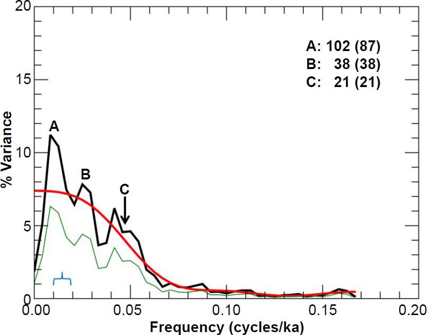
Fig. 9. Unprewhitened RC11-120 (southern hemisphere) summer sea surface temperature power spectrum. Numbers in bold indicate the periods (in ka) of prominent spectral peaks, and numbers in parentheses are the periods originally reported in the Pacemaker paper. The smooth red curve represents the null continuum, the light green line represents the lower bound of the 80% confidence interval, and the blue bracket indicates the approximate bandwidth.

As noted earlier, I have also included the null continua and the lower bounds of the 80% confidence intervals to help the reader get a feel for the height of spectral peaks compared to the backgrounds. The reason for doing so should hopefully become apparent in Part III of this series, although I recognize that a rigorous analysis of statistical significance must be postponed until prewhitening. I have also included a light blue bracket to indicate the approximate equivalent bandwidth (width of the bracket may disagree slightly with the calculated bandwidth, due to resolution limitations), after Eq. (35). A value of m = 7 was used to obtain the null continua for all three variables in the RC11-120 core. Note that their percentage variance values are about half of mine; the Pacemaker authors apparently plotted Γ(f), rather than P(f), in their Fig. 5.

Overall, there is good agreement between the shapes of my spectra and theirs, as well as generally good agreement between the periods of my dominant peaks and theirs. Although I have not received legal permission to reproduce their results in this paper (reproduction of figures from Science papers published between 1974 and 1994 require the author’s permission, and my request for this permission went unanswered), an internet search should quickly locate a picture of their Fig. 5, so that their results may be compared with mine.

Despite the generally good visual match between my results and theirs, in some cases there is noticeable disagreement. For instance, there are some noticeable differences between my Fig. 11 and their chart in the upper right-hand corner of their Fig. 5 (the RC11-120 spectrum results for % C. davisiana). The trough between peaks A and B in my Fig. 11 is not as deep as it was in Pacemaker. Likewise, they did not report a period value for my peak C, since their graph exhibits more of a plateau than a peak at that location. There were also some differences between my reported peak periods and theirs. My period of 119 ka for peak A in Fig. 11 is noticeably larger than their reported value of 106 ka. However, my period of 102 ka for peak A in Fig. 9 is actually a better match to the expected 100 ka value than the originally reported value of 87 ka. The same is true for my peak A in Fig. 10.

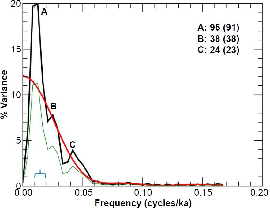
Fig. 10. Unprewhitened RC11-120 oxygen isotope power spectrum. Numbers in bold indicate the periods (in ka) of prominent spectral peaks, and numbers in parentheses are the periods originally reported in the Pacemaker paper. The smooth red curve represents the null continuum, the light green line represents the lower bound of the 80% confidence interval, and the blue bracket indicates the approximate bandwidth.

---

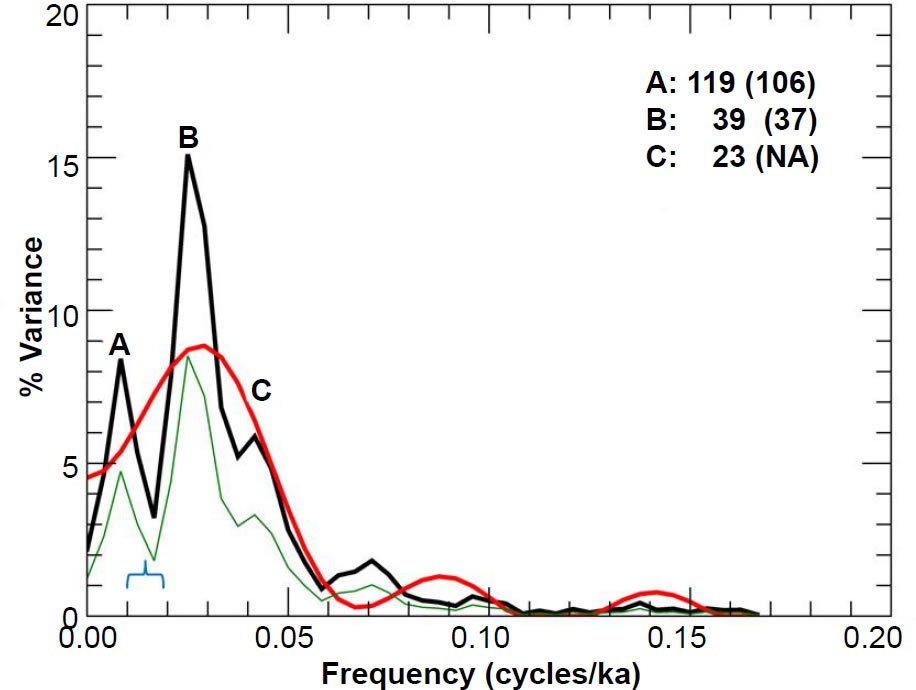
Fig. 11. Unprewhitened RC11-120 %. C. davisiana power spectrum. Numbers in bold indicate the periods (in ka) of prominent spectral peaks, and numbers in parentheses are the periods originally reported in the Pacemaker paper. The smooth red curve represents the null continuum, the light green line represents the lower bound of the 80% confidence interval, and the blue bracket indicates the approximate bandwidth.

Also, my peaks tend to not be as sharp as those in the original Pacemaker paper. Some of this may be due to the inherent error of attempting to reconstruct the data from Figs. 2 and 3 in Pacemaker.

Replication of Results: E49-18

Likewise, my unprewhitened spectral results for the E49-18 core (using the SIMPLEX chronology) are shown in Figs. 12–14. Per the Pacemaker paper, I also used a time increment of Δt = 3 ka. Interpolation resulted in n = 122 data points. As before, this was one greater than their reported value of n = 121, but my interpolated timescale extends from t = 127 ka to t = 490 ka, in very good agreement with their reported timescale of 127–489 ka.

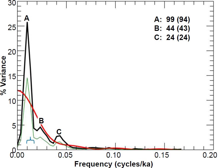
Fig. 12. Unprewhitened E49-18 summer sea surface temperature power spectrum. Numbers in bold indicate the periods (in ka) of prominent spectral peaks, and numbers in parentheses are the periods originally reported in the Pacemaker paper. The smooth red curve represents the null continuum, the light green line represents the lower bound of the 80% confidence interval, and the blue bracket indicates the approximate bandwidth.

---

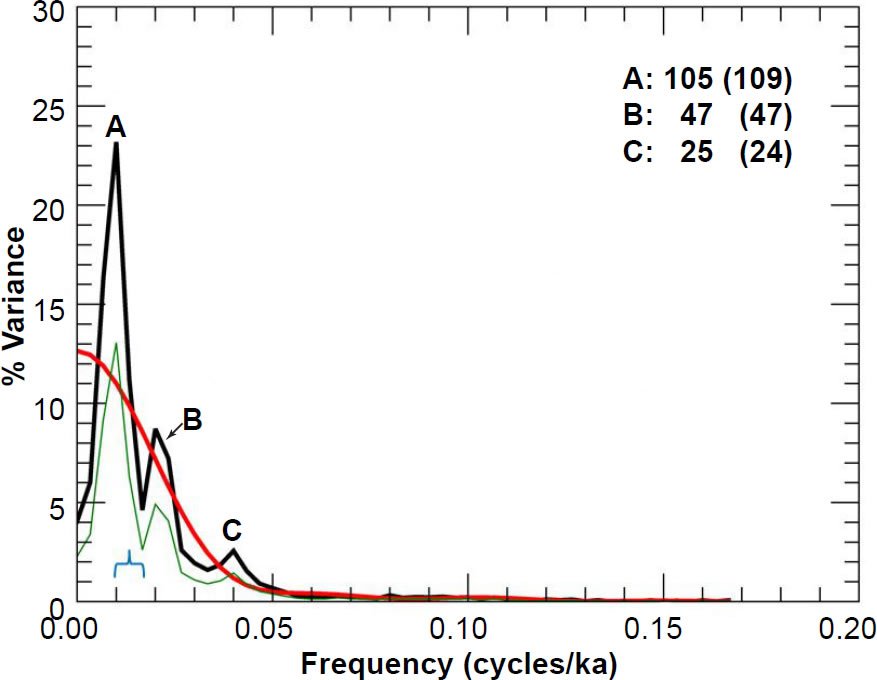
Fig. 13. Unprewhitened E49-18 oxygen isotope power spectrum. Numbers in bold indicate the periods (in ka) of prominent spectral peaks, and numbers in parentheses are the periods originally reported in the Pacemaker paper. The smooth red curve represents the null continuum, the light green line represents the lower bound of the 80% confidence interval, and the blue bracket indicates the approximate bandwidth.

---

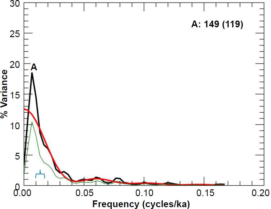
Fig. 14. Unprewhitened E49-18 % C. davisiana power spectrum. Number in bold indicates the period (in ka) of the prominent spectral peak, and the number in parentheses is the period originally reported in the Pacemaker paper. The smooth red curve represents the null continuum, the light green line represents the lower bound of the 80% confidence interval, and the blue bracket indicates the approximate bandwidth.

I chose m = 8 to obtain the null continua, as this choice seems to give the best overall null continua estimates for all three variables. As in the case of the RC11-120 spectra, I have also included the lower bounds of the 80% confidence intervals in my graphs. There is a generally good visual match between my reproduced spectra and those depicted in the second row of Fig. 5 in Pacemaker. However, there is a major discrepancy between their reported period of 119 ka for the dominant A peak in the % C. davisiana power spectrum and my value (Fig. 14) of 149 ka.

Very little truncation was required in this case. Only three high-frequency spectral values within the E49-18 δ¹⁸O power spectrum were slightly negative.

Replication of Results: PATCH

Finally, I include in Figs. 15–17 the power spectra for the ELBOW chronology and the PATCH records, obtained by appending data from the top 785 cm in the RC11-120 core to the data below 825 cm in the E49-18 core. The Pacemaker authors thought they could do this because the depth of 785 cm in the RC11-120 core and the depth of 825 cm in the E49- 18 core both corresponded to the presumed MIS 8-7 boundary, to which they assigned an age of 251 ka. Figs. 15–17 correspond to the third row of charts in their Fig. 5. In order to obtain their null continua in a later part of the paper, the authors set m = 8 (Hays, Imbrie, and Shackleton 1976, 1132, endnote no. 57), although I think m = 7 gives an overall better fit for the prewhitened results (discussed in a later paper). This discrepancy could be due to slight differences between the original and my reconstructed data sets. Again, there is generally favorable agreement between my results and those in Pacemaker.

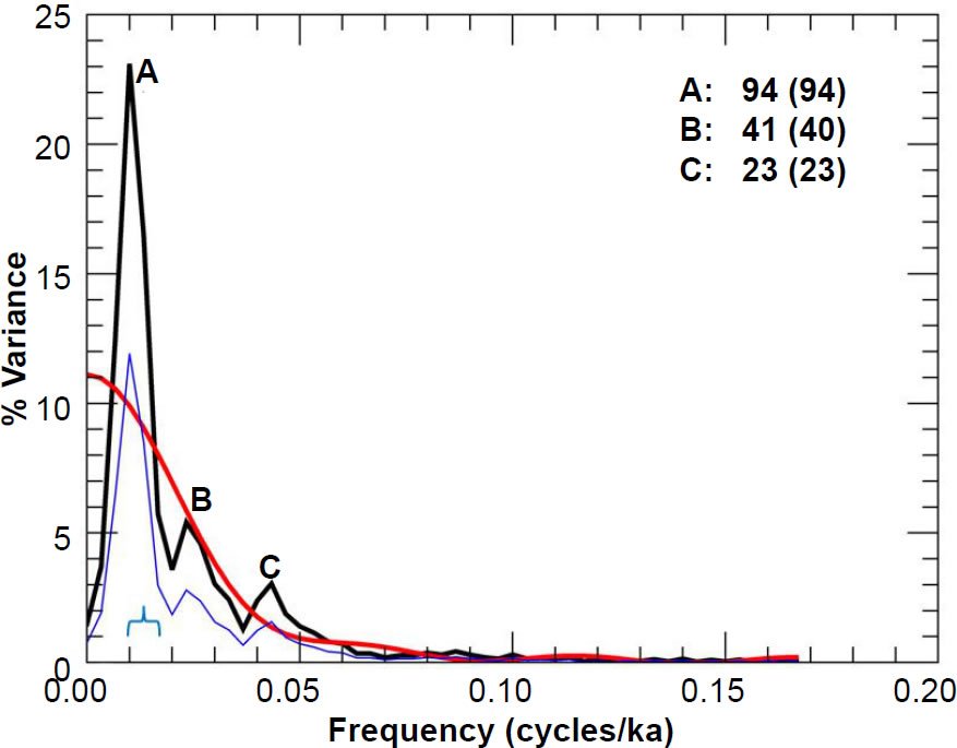
Fig. 15. Unprewhitened PATCH summer sea surface temperature power spectrum. Numbers in bold indicate the periods (in ka) of prominent spectral peaks, and numbers in parentheses are the periods originally reported in the Pacemaker paper. The smooth red curve represents the null continuum, the light blue line represents the lower bound of the 90% confidence interval, and the blue bracket indicates the approximate bandwidth.

---

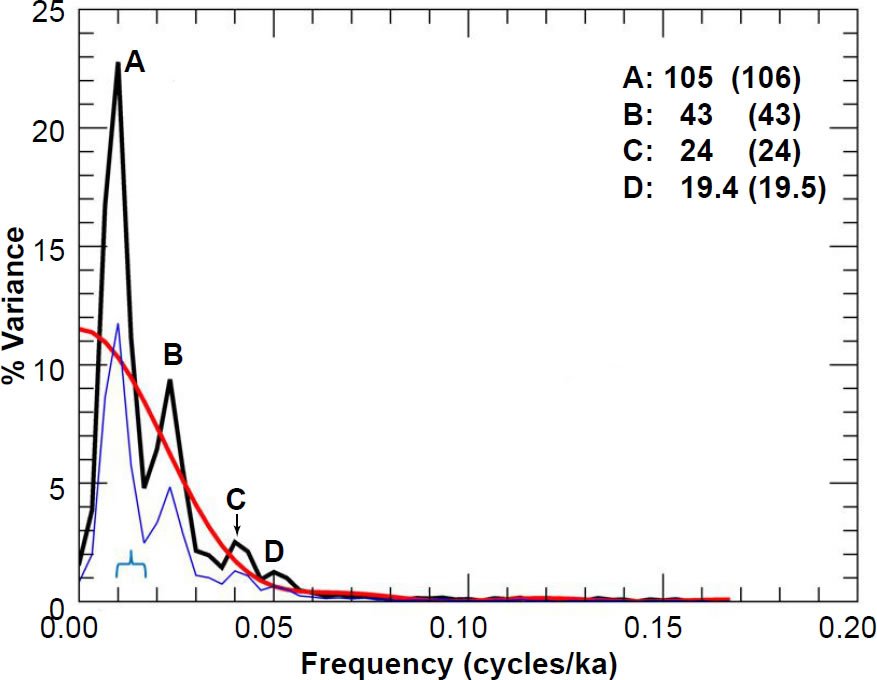
Fig. 16. Unprewhitened PATCH oxygen isotope power spectrum. Numbers in bold indicate the periods (in ka) of prominent spectral peaks, and numbers in parentheses are the periods originally reported in the Pacemaker paper. The smooth red curve represents the null continuum, the light blue line represents the lower bound of the 90% confidence interval, and the blue bracket indicates the approximate bandwidth. The “D” peak is not labelled in Fig. 5 of Pacemaker, but it is listed in that paper’s Table 4.

---

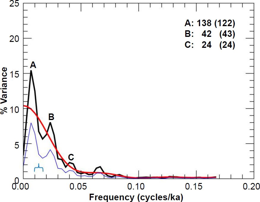
Fig. 17. Unprewhitened PATCH % C. davisiana power spectrum. Numbers in bold indicate the periods (in ka) of prominent spectral peaks, and numbers in parentheses are the periods originally reported in the Pacemaker paper. The smooth red curve represents the null continuum, the light blue line represents the lower bound of the 90% confidence interval, and the blue bracket indicates the approximate bandwidth.

Only one high-frequency spectral value within the PATCH δ¹⁸O power spectrum needed to be truncated, as well as four values in the high-frequency portion of the PATCH SST null continuum.

For the three PATCH spectra, I have also plotted the lower bounds of the 90% confidence intervals.

Summary

Now that we have explained the Blackman-Tukey method and demonstrated that my code can replicate, using the same multi-step procedure described by the Pacemaker authors, the original results with a good deal of precision, it is now time to discuss in Part III of this series the statistical significance of the original results, as well as the effect of the new age assignment for the B-M reversal on the resulting power spectra. We also discuss the effect of including all the E49-18 data in the analysis. Unfortunately for proponents of Milankovitch climate forcing, these effects are quite negative.

References

Anava, O., E. Hazan, S. Mannor, and O. Shamir. 2013. “Online Learning for Time Series Prediction.” Journal of Machine Learning Research: 2013 Workshop and Conference Proceedings: 1–13.

Arfken, G. B., and H. J. Weber. 2005. Mathematical Methods for Physicists. 6th ed. Amsterdam, The Netherlands: Elsevier.

Blackman, R. B., and J. W. Tukey. 1958. The Measurement of Power Spectra from the Point of View of Communications Engineering. New York, New York: Dover Publications.

Buttkus, B. 2000. Spectral Analysis and Filter Theory in Applied Geophysics. English ed. Berlin, Germany: Die Deutsche Bibliothek.

Cronin, T. M. 2010. Paleoclimates: Understanding Climate Change Past and Present. New York, New York: Columbia University Press.

Gilman, D. L., F. J. Fuglister, and J. M. Mitchell, Jr. 1963. “On the Power Spectrum of ‘Red Noise’.” Journal of the Atmospheric Sciences 20 (2): 182–184.

Hartmann, D. L. 2013. Classroom Notes for Spectral Analysis. http://www.atmos.washington.edu/~dennis/552_Notes_6b.pdf.

Hayes, J. D., J. Imbrie, and N. J. Shackleton. 1976. “Variations in the Earth’s Orbit: Pacemaker of the Ice Ages.” Science 194 (4270): 1121–1132.

Hebert, J. 2014. “Circular Reasoning in the Dating of Deep Seafloor Sediments and Ice Cores: The Orbital Tuning Method.” Answers Research Journal 7: 297–309.

Hebert, J. 2015. “The Dating ‘Pedigree’ of Seafloor Sediment Core MD97-2120: A Case Study.” Creation Research Society Quarterly 51 (3): 152–164.

Hebert, J. 2016. “Revisiting an Iconic Argument for Milankovitch Climate Forcing: Should the ‘Pacemaker of the Ice Ages’ Paper Be Retracted? Part I.” Answers Research Journal 9: 25–56.

Honerlaw, M. n.d. Purdue University Statistics class notes. http://www.stat.purdue.edu/~mhonerla/stat301/Chapter_7.pdf.

Hu, L. 2006. Lecture 1: Stationary Time Series. Lecture Notes for Ohio State University Economics Class. http://www. econ.ohio-state.edu/dejong/note1.pdf.

Imbrie, J. 1982. “Astronomical Theory of the Pleistocene Ice Ages: A Brief Historical Review.” Icarus 50 (2–3): 408–422.

Imbrie, J., and N. Pisias. n.d. Climap Handbook of Time-Series Analysis. Archived as Columbia University class notes for Cenozoic Paleoceanography course (as of 10/27/2015). http://eesc.columbia.edu/courses/w4937/Readings/Climap_handbook_Time_Series.pdf.

Jenkins, G. W., and D. G. Watts. 1968. Spectral Analysis and Its Applications. San Francisco, California: Holden-Day.

Kanasewich, E. R. 1985. Time Sequence Analysis in Geophysics. 3rd ed. Alberta, Canada: University of Alberta Press.

Khintchin, A. 1934. “Korrelationstheorie der stationären stochastischen Prozesse.” Mathematische Annalen 109 (1): 604–615.

Mann, M. E., and J. M. Lees. 1996. “Robust Estimation of Background Noise and Signal Detection in Climatic Time Series.” Climatic Change 33 (3): 409–445.

Mayo, D. G. 1981. “In Defense of the Neyman-Pearson Theory of Confidence Intervals.” Philosophy of Science 48 (2): 269–280.

Meko, D. 2015. University of Arizona Classroom notes for Dendrochronology 585A. http://www.ltrr.arizona.edu/~dmeko/notes_6.pdf.

Meyers, S. R. 2012. “Seeing Red in Cyclic Stratigraphy: Spectral Noise Estimation for Astrochronology.” Paleoceanography 27 (3): 1–12.

Milankovic, M. 1941. Canon on Insolation and the Ice-Age Problem. Belgrade, Serbia: Special Publications of the Royal Serbian Academy, vol. 132.

Mudelsee, M. 2002. “TAUEST: A Computer Program for Estimating Persistence in Unevenly Spaced Weather/ Climate Time Series.” Computers and Geosciences 28 (1): 69–72.

Muller, R. A., and G. J. MacDonald. 2000. Ice Ages and Astronomical Causes: Data, Spectral Analysis and Mechanisms. Chichester, United Kingdom: Praxis Publishing.

Nason, G. 2014. Tests of Stationarity. University of Bristol School of Mathematics. http://www.maths.bris.ac.uk/~guy/Research/LSTS/TOS.html.

Oard, M. J. 2007. “Astronomical Troubles for the Astronomical Hypothesis of Ice Ages.” Journal of Creation 21 (3): 19–23.

Press, W. H., S. A. Teukolsky, W. T. Vetterling, and B. P. Flannery. 2007. Numerical Recipes: The Art of Scientific Computing. 3rd ed. Cambridge, United Kingdom: Cambridge University Press.

Schulz, M., and M. Mudelsee. 2002. “REDFIT: Estimating Red- Noise Spectra Directly from Unevenly Spaced Paleoclimatic Time Series.” Computers and Geosciences 28 (3): 421–426.

Spiegel, M. R. 1994. Schaum’s Outline Series: Mathematical Handbook of Formulas and Tables. 3rd ed. New York, New York: McGraw-Hill.

Thomas, G. B. Jr., and R. L. Finney. 1988. Calculus and Analytic Geometry. 7th ed. Reading, Massachusetts: Addison-Wesley.

Thomson, R. E., and W. J. Emery. 2014. Data Analysis Methods in Physical Oceanography. 3rd ed. Amsterdam, The Netherlands: Elsevier.

Walker, M., and J. Lowe. 2007. “Quaternary Science 2007: A 50-Year Retrospective.” Journal of the Geological Society, London 164 (6): 1073–1092.

Weedon, G. P. 2003. Time-Series Analysis and Cyclostratigraphy: Examining Stratigraphic Records of Environmental Cycles. Cambridge, United Kingdom: Cambridge University Press.

Wiener, N. 1930. “Generalized Harmonic Analysis.” Acta Mathematica 55 (1): 117–258.

Wunsch, C. 2010. Time Series Analysis: A Heuristic Primer. Classroom Notes. http://isites.harvard.edu/fs/docs/icb.topic719287.files/time_series_primer_22jan2010.pdf.