
The views expressed in this paper are those of the writer(s) and are not necessarily those of the ARJ Editor or Answers in Genesis.
Abstract
The “Pacemaker of the Ice Ages” paper by Hays, Imbrie, and Shackleton (1976) convinced the secular scientific community of the validity of the modern version of Milankovitch climate forcing. Power spectrum analyses performed on (presumed) climatically significant variables from two Indian Ocean sediment cores showed dominant spectral peaks at frequencies corresponding to orbital cycles within the Milankovitch hypothesis. However, this paper, the first in a series of papers, demonstrates that much of the Hays et al. paper, as originally presented, is invalid (even within a uniformitarian framework) and that it arguably should be retracted. First, Hays et al. omitted nearly one-third of all the available data from the E49-18 core on the grounds that much of the core top was missing, a claim since disputed by other uniformitarian scientists. Second, one of the key dates used by Hays et al. to establish timescales for the cores, an assumed age of 700,000 years for the Brunhes-Matuyama (B-M) magnetic reversal boundary, is significantly lower than the currently accepted age of 780,000 years. This new age assignment is extraordinarily problematic for the paper, as discussed below. Finally, the data sets used in the analysis have “evolved” over the years, raising the question, which versions of the data are the “real” ones?
Introduction
The well-known “Pacemaker of the Ice Ages” paper (Hays, Imbrie, and Shackleton 1976, hereafter referred to as Pacemaker) is largely responsible for today’s wide acceptance among uniformitarian scientists of the hypothesis of Milankovitch-induced climate forcing.
The Milankovitch (or astronomical) hypothesis of Pleistocene ice ages is now the dominant explanation for the 50 or so Pleistocene glacial intervals (“ice ages,” in popular speech) that have supposedly occurred within the last 2.6 million years (Walker and Lowe 2007). It was first proposed by J. A. Adhémar and James Croll in the 1800s but was later refined by Serbian geophysicist Milutin Milanković (Imbrie 1982; Milanković 1941). Supposedly, glacial intervals are caused by decreases in northern hemisphere summer high latitude sunlight, which are themselves caused by slow variations in the earth’s orbital and rotational motions. The most obvious problem with the Milankovitch hypothesis is that it is not clear how ice ages can plausibly be caused by very small decreases in high latitude solar insolation.
The hypothesis also suffers from other difficulties (Oard 2007), many of which are acknowledged even by secular scientists (Cronin 2010, 130–39). Nevertheless, uniformitarian scientists generally assume the Milankovitch hypothesis to be correct and use it to assign ages to the seafloor sediments via a technique called orbital tuning (Cronin 2010; Hebert 2014, 2015; Herbert 2010). In fact, uniformitarian scientists are now using Milankovitch cycles to extend an astronomical timescale in sedimentary rocks all the way back to the beginning of the Triassic Period (Hinnov and Hilgen 2012).
Despite the fact that the Milankovitch hypothesis had been rejected by previous generations of scientists (Imbrie 1982, 415–16), it is now widely accepted largely as the result of Pacemaker. The paper’s authors performed power spectrum analyses on data having presumed climatic significance: planktonic foraminiferal oxygen isotope ratios, the relative abundance of one particular radiolarian species, and estimated sea surface temperature data (also inferred from radiolarian data) from the two Indian Ocean sediment cores RC11-120 and E49-18 (Fig. 1). When these data are plotted as a function of depth, many wiggles, with occasional prominent peaks and troughs become apparent. Oxygen isotope wiggles for the RC11-120 core are illustrated in Fig. 2. Largely because the power spectra of these data showed dominant spectral peaks at frequencies corresponding to dominant cycles within the Milankovitch hypothesis, the paper was seen as providing strong support for the Milankovitch hypothesis. The importance of this seminal paper is illustrated by the following comment by (Dietrich 2011, 17): “It was not until the advent of deep-ocean cores and the seminal paper by Hays, Imbrie, and Shackleton—‘Variations in the Earth’s Orbit: Pacemaker of the Ice Ages’ in Science (1976) that astronomical-climate theories became accepted.”
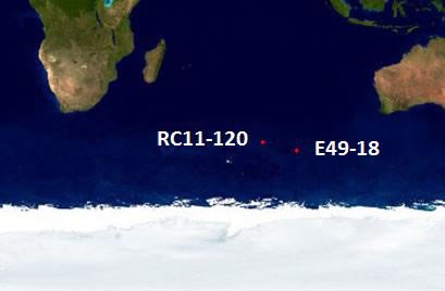
Fig. 1. The Pacemaker paper by Hays, Imbrie, and Shackleton (1976) used data from Indian Ocean deep-sea sediment cores RC11-120 and E49-18.
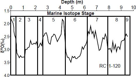
Fig. 2. My reconstructed values (from Table A1 in the appendix) of the RC11-120 oxygen isotope values from the Pacemaker paper, along with the approximate marine isotope stage (MIS) boundary locations.
This view is shared by (Muller and MacDonald 2000, xiv):
In fact, the evidence for the role of astronomy [in climate variation] comes almost exclusively from spectral analysis. The seminal paper was published in 1976, titled, “Variations of [sic] the earth’s orbit: pacemaker of the ice ages” (Hays et al., 1976).
In fact, in his Foreword to the previous reference, (Muller and MacDonald 2000, xvii), Walter Alvarez goes even further than Muller and MacDonald: “The widely accepted Croll-Milankovitch theory that fluctuating climate conditions during the Quaternary glaciation have been driven by astronomical cycles is based entirely on time-series analysis of paleoclimatic and orbital data.” (emphasis mine)
Because of the great importance of Pacemaker, it is definitely worthwhile to reexamine it in detail. Before one can discuss potential problems with the paper, however, it is necessary to first discuss the relevant background material. Readers already familiar with the Milankovitch hypothesis, oxygen isotope ratios, marine isotope stages, the Termination II causality problem, and orbital tuning may wish to skip ahead to the section entitled “Pacemaker Problems: Needlessly Excluded Data?”
Milankovitch Orbital Cycles
The Milankovitch (or astronomical) hypothesis posits that subtle changes in the seasonal and latitudinal distribution of sunlight have “paced” the Pleistocene ice ages and, by extension (according to current uniformitarian thinking noted earlier), have also paced the deposition of the sedimentary record even hundreds of millions of years prior. The amount of summer sunlight at 65°N is generally considered to be the “driver” for these climate variations, although others have argued that sunlight variations at other latitudes and seasons are actually responsible (Cronin 2010, 119; Muller and Macdonald 2000, 39). These changes in solar insolation are in turn thought to be caused by changes in the earth’s orbital and rotational motions, occurring slowly over many tens of thousands of years.
For instance, the earth’s rotational axis is tilted at an angle of 23.4° from a line perpendicular to the plane of the earth’s orbit around the sun (the ecliptic). However, this angle is slowly changing, with a minimum value of 22.1° and a maximum value of 24.5°. Since secular scientists believe the solar system is billions of years old, they feel free to extrapolate this slow, subtle motion backward into the presumed “prehistoric” past. Given that assumption, it would take about 41,000 years for the earth’s axial tilt, or obliquity, to change from 22.1° to 24.5° and back again.
Likewise, the shape of the earth’s orbit is slowly changing, becoming slightly less elliptical over time. This causes the earth’s perihelion and aphelion to move a little closer and farther away from the sun over time.
This change in the shape of the earth’s orbit is characterized by cycles with periods of about 405 and 100 ka. Actually, Milankovitch insolation theories predict that the 100 ka cycle should actually be composed of two cycles (Muller and MacDonald 2000, 13):
The attention given to spectrum shape has created another serious problem for the insolation theory. A high-resolution analysis of the 100 kyr cycle shows that the insolation theory, and its variants, all predict that the peak will have a split structure: it will be resolved into a 95 kyr line and a 125 kyr line. (An exception to this general rule is a model recently published by W. Berger, and explained in Section 6.4.8.) The bulk of the data shows that this prediction is contradicted. The 100 kyr cycle is a single narrow line. Ad hoc mechanisms that were plausible for eliminating the 400 kyr line are not plausible for turning the predicted doublet into a singlet. It is remarkable that this problem was not noticed until 1994.
Muller and MacDonald have suggested that the 100 ka cycle may not be the result of changes in eccentricity, but are instead related to changes in earth’s orbital inclination, the angle between the plane of the ecliptic and the plane perpendicular to the angular momentum vector of the planets (Muller and MacDonald 2000, 40–45). Since changes in inclination should not affect insolation, they suggest that changes in inclination may cause the earth’s orbit to pass through different regions of meteoroids and dust, and that these small particles affect earth’s climate. However, they acknowledged that their proposed mechanism is speculative, and that there are as yet no known meteoroid or dust bands that meet all the necessary conditions for their hypothesis to be valid (Muller and MacDonald 1997, 8332).
Gravitational forces exerted on the earth’s equatorial bulge by the sun and moon cause a torque that results in a wobble of the earth’s rotational axis, much like the wobble of a spinning top. This precession has a period of about 26 ka.
In addition to the change in shape of the earth’s orbit, orbital precession caused by gravitational interactions between the earth and the other planets is also causing this orbit to slowly rotate relative to the background stars. Precession and orbital precession together combine to yield an overall cycle of about 23 ka during which aphelion and perihelion advance through the seasons of the year.
Hence, according to the Milankovitch hypothesis, one might expect earth’s climate to be cyclic, alternating between ice ages and warmer interglacials every 405,000, 100,000, 41,000, or 23,000 years. Since Pacemaker purported to show evidence for the last three of these cycles, it is viewed as having confirmed the Milankovitch hypothesis. Examination of Figs. 5 and 6 in Pacemaker show that the spectral peaks corresponding to periods of ~100 ka are generally much more prominent than the peaks corresponding to the 41 and 23 ka cycles. Yet according to solar insolation calculations, variations in the distribution of sunlight due to the eccentricity cycle are extremely small. Hence, of all the astronomical cycles, the eccentricity cycle should have the weakest effect on climate. This “100-ka enigma” is just one of several puzzling features of the modern version of the Milankovitch hypothesis (Cronin 2010, 130–31).
The Oxygen Isotope Ratio
Paleoclimatologists view the oxygen isotope ratio as a climate indicator.
There are three stable isotopes of the oxygen atom: oxygen-16, oxygen-17, and oxygen-18. Oxygen-17 is extremely rare relative to the other two isotopes and will not be mentioned again in this discussion. Oxygen-16 is about 500 times more abundant than the slightly heavier oxygen-18 isotope. The oxygen isotope ratio, denoted by the symbol δ18O, is a measure of the amount of oxygen-18 compared to oxygen-16 within a sample, relative to a standard oxygen isotope value (Wright 2010). The oxygen isotope value is calculated by the formula
Because 18O is much less abundant than 16O, δ18O values are multiplied by 1000 in order to prevent them from being inconveniently small. They are then expressed in units of “per mil” (per thousand) or “‰”. Higher oxygen isotope values indicate an enhancement of oxygen-18 compared to oxygen-16 (relative to the standard), while lower oxygen isotope values indicate a decrease in oxygen-18 compared to oxygen-16 (also relative to the standard).
Oxygen isotope values may be measured for shells (or tests) of marine-dwelling protists called foraminifera (“forams” for short), since these shells are composed of oxygen-containing calcite, or calcium carbonate (CaCO3). Foraminifera are generally classified as either planktonic or benthic. Planktonic forams are free-floating (Mortyn and Charles 2003), while benthic forams dwell on and within the seafloor sediments (Kingston 2010). When the forams die, their shells (tests) become part of the seafloor sediments accumulating on the ocean floor.
An empirically determined relationship (Epstein et al. 1953) between the seawater temperature T at the time of foraminifera shell formation, the δ18O value of the calcite itself, and the δ18O value of the surrounding seawater is given by
Although paleoclimatologists view foraminiferal δ18O values within the seafloor sediments as a climate indicator, the precise meaning attributed to these δ18O values has changed over the years. Cesare Emiliani, a founding father of paleoceanography, claimed that δ18Ocalcite values could act as a paleothermometer, with most of the variation in these values resulting from temperature changes (Emiliani 1966). Nicholas Shackleton argued that this view was implausible and that most of the variation in sediment δ18O values was due instead to variations in the amount of global ice cover (Shackleton 1967). This view is now the consensus interpretation (Walker and Lowe 2007; Wright 2010).
Marine Isotope Stages
As previously noted, if one plots oxygen isotope values from a sediment core as a function of depth, one will observe many wiggles, with occasional prominent peaks and troughs. In fact, this is also true for other quantities that could be measured within the core, such as estimated sea surface temperatures. Relatively high and low foram δ18O values are thought to indicate colder and warmer climates, respectively. More precisely, the highest values of δ18O within a sediment core are thought to indicate times of maximum glacial extent, and the smallest values are thought to indicate times of minimum glacial extent.
Because uniformitarian paleoclimatologists believe that changes in δ18O values are indicative of global climate variations, they have devised a numbering system to identify prominent features in the δ18O signal which should, in principle, be present in every sediment core (assuming a sufficiently long core length, minimal core disturbance, and a sufficiently high signal-to-noise ratio). Secular paleoclimatologists use a numbering system called marine isotope stages (MIS) to identify the alternating warm and cold periods that they believe are indicated by the wiggles. Warmer periods are generally (but with some exceptions) identified by odd numbers, starting with a 1 for today’s climate, thought to be the most recent of many warm interglacials. Colder periods are generally indicated by even numbers, beginning with a 2 for the end of the most recent ice age. Boundaries between these stages are usually placed at the midpoints between presumed temperature maxima and minima (Gibbard 2007).
The approximate locations of the presumed Marine Isotope boundaries for the RC11-120 core are shown in Fig. 2 (after Hays, Imbrie, and Shackleton 1976). Note the inverted scale on the vertical axis: minimum δ18O values appear near the top of the graph, and maximum δ18O values appear near the bottom. Hence the δ18O “peaks” in Fig. 2 are thought to represent times of minimum ice volume, and the δ18O “troughs” are believed to represent times of maximum ice volume.
The Termination II Causality Problem
A termination within an ice or sediment core is defined to be the oxygen isotope ratio that represents the midpoint between full glacial and full interglacial conditions (Broecker and Henderson 1998, 352). As we have already seen, these terminations (Broecker and van Donk 1970, 171) generally mark the boundaries between the marine isotope stages (Gibbard 2007).
Termination II (T-II) is the name given to the end of the penultimate (second-to-last) glacial interval (Siddall et al. 2006), thought to have occurred roughly 130,000 years ago (Shakun et al. 2011, 1). Although one might expect from Fig. 2 that the penultimate glacial interval would correspond to MIS 4, uniformitarian paleoclimatologists consider MIS 2-4 to be a single glacial interval (Wolff et al. 2010, 2828); hence the end of the penultimate glacial interval actually corresponds to the MIS 6-5 boundary.
The manner in which terminations have been defined implies that Termination II is the MIS 6-5 boundary.
The causality problem refers to the fact that some data sets (Karner and Muller 2000; Winograd et al. 1992) seem to imply that the transition from the MIS 6 glacial to the MIS 5 interglacial occurred about 133–145 ka ago, even though the increases in high latitude summer sunlight that supposedly caused this transition should have occurred ~130,000 years ago, according to Milankovitch expectations. In other words, the effect appears to precede the cause by multiple thousands of years, an obvious problem for the Milankovitch hypothesis.
Orbital Tuning
Because most seafloor sediments contain low amounts of heavy radioactive elements, radioisotopic dating methods cannot generally be used to directly date the seafloor sediments (although the Protactinium-231/Thorium-230 dating method is thought to be sometimes capable of dating relatively young sediments (Cheng et al. 1998) with ages beyond the range of radiocarbon dating. However, radioisotope dating may be used to assist in this process by assigning ages to magnetic reversal boundaries recorded in volcanic rocks. Once an age has been assigned to the reversal boundary, this age may be transferred to depths within cores that mark the location of this particular reversal. Likewise, radiocarbon dating may be used to assign ages to the uppermost sediments. In order to assign ages to other depths within the core, paleoclimatologists must construct an age-depth model that makes assumptions about past sedimentation rates.
The simplest possible age-depth model for a seafloor sediment core would assume that sediments at that location have been deposited at a perfectly constant rate throughout earth history (Herbert 2010, 370). Such a model would also ignore possible complications such as compaction of the sediments, disturbance of the sediments by ocean currents, or disturbance of the sediments by marine organisms (bioturbation). However, even uniformitarian scientists do not believe that past earth processes have been that uniform! Rather, they believe that sedimentation rates, though slow and gradual, have varied somewhat in the past, with some times characterized by sedimentation rates that were higher-than-average and some that were lower-than-average. They use the technique of orbital tuning to determine the presumed changes in these past rates, as well as the ages assigned to the seafloor sediments.
Although the orbital tuning method may utilize different mathematical techniques, the conceptual heart of the method is fairly simple: adjust the timescale for the sediment core so that the wiggles match expectations of the Milankovitch hypothesis. This can be done via a variety of methods (Muller and MacDonald 2000, 141–44).
The tuning process distorts the δ18O signal somewhat, causing some of the wiggles to be stretched and others to be compressed. Fig. 3 demonstrates this accordion-like compression and expansion, using actual benthic δ18O values from the Atlantic DSDP 607 core. These data and the timescale for the core were obtained from ftp://ftp.ncdc.noaa.gov/pub/data/paleo/contributions_by_author/raymo1989/raymo1992.txt (the fifth listed data set) on 4/23/2015. The data archived there were compiled from multiple sources, including Boyle and Keigwin (1985), Cande and Kent (1992), Mix and Fairbanks (1985), Raymo (1992), Raymo et al. (1989), Ruddiman et al. (1989), and Shackleton, Berger, and Peltier (1990).
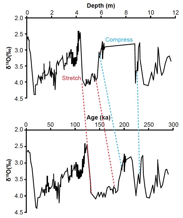
Fig. 3. Illustration of the stretching and compressing of seafloor sediment core data resulting from the orbital tuning process. Diagram uses actual benthic oxygen isotope data from the Atlantic DSDP 607 core.
However, it is important to realize that, in the absence of clear evidence for the validity of the Milankovitch hypothesis, orbital tuning is nothing more than circular reasoning, as even randomly generated signals can be forced to agree with the Milankovitch hypothesis (Neeman 1993). Other uniformitarian scientists have also pointed out the potential dangers in tuning methods (Blaauw 2010; Blaauw, Bennett, and Christen 2010).
This is why the Pacemaker paper is so important: because the paper was seen as having confirmed the Milankovitch hypothesis, uniformitarian paleoclimatologists now feel free to assume the validity of Milankovitch climate forcing, and to use that assumption to date other seafloor sediments via the orbital tuning process. Furthermore, the ages assigned to sediment cores are then used to date still other sediment cores, as well as to assign ages to the deep ice cores of Antarctica and Greenland (Hebert 2014, 2015).
Potential Problems with Inferring Climate Data from Sediments
Also, as indicated by equation (2), foraminiferal oxygen isotope values, which are thought to serve as a proxy for global ice volume, depend upon both the temperature and the oxygen isotope value of the surrounding seawater at the time of calcite formation. Neither of these (past) variables can be measured in the laboratory. Likewise, melting of the ice sheets would influence ocean δ18O values, due to the large sizes of the ice sheets and their low δ18O values compared to that of seawater (Wright 2010, 320). But high latitude ice sheet volume also depends on temperature. How then does one separate these two effects when interpreting the foraminiferal δ18O data? Likewise, temperature itself is a function of both global climate and local effects. How then does one deconvolve which part of the temperature is due to the global climate and which part is due to local effects? Paleoceanographers will often stack data from multiple cores in an attempt to obtain an average signal that minimizes locally induced noise in individual cores (Lisiecki and Raymo 2005), but this process requires data from multiple cores. For instance, although the Pacemaker authors combined data from two different cores in order to produce a longer composite core, their procedure did not reduce possible noise via an averaging process. Karner et al. (2002, 1) have acknowledged that the noise from local effects is a potential problem for Pacemaker. This problem is especially acute for studies using planktonic foraminifera (such as Pacemaker), because planktonic foraminifera are free-floating and are more likely to be influenced by spatial and temporal variations in temperature. A good (albeit dated) overview of the problems confronting attempts to infer past climates from foraminiferal δ18O values is found in Oard (1984).
Orbital Tuning and Circular Reasoning
Of course, if the Milankovitch hypothesis is wrong, then the orbital tuning technique is invalid, and uniformitarian scientists are simply engaging in circular reasoning. They have recognized this potential for circular reasoning (Herbert 2010, 372) and attempt to guard against it. For instance, they may write computer algorithms to perform the tuning in an attempt to remove subjectivity from the process. They may also incorporate within these algorithms penalties for tuned timescales that require extreme sedimentation rates or extreme changes in sedimentation rates (Lisiecki and Raymo 2005, 3). Although these techniques may be able to distinguish between reasonable and unreasonable sedimentation histories within a uniformitarian worldview, they have already assumed an old earth and have excluded the biblical history from serious consideration.
Now that we have discussed the necessary background material, we are now prepared to discuss specific problems with the Pacemaker paper in more detail.
Pacemaker Problems: Needlessly Excluded Data?
First, this putative confirmation of the Milankovitch hypothesis involved only two sediment cores, and not even two complete cores at that. The Pacemaker authors omitted nearly a third of all the available E49-18 data from their analysis, claiming that much of the upper core section had been disturbed as a result of scouring by bottom currents. They estimated that the top of the E49-18 core could be as old as 60,000 years (Hays, Imbrie, and Shackleton 1976, 1123). The Pacemaker authors refrained from using the upper 4.9 m of the E49-18 core in their analysis, citing this uncertainty in age for the top of the core.
However, there are two serious problems with their exclusion of these data. First, the exclusion of data from the top of E49-18 was based almost entirely on the relative abundance of one particular radiolarian species, Cycladophora davisiana. In another paper published that same year, Hays et al. (1976) analyzed radiolarian data from multiple Antarctic and sub-Antarctic sediment cores. They argued that a particularly high relative abundance of C. davisiana (~20–30%) occurred roughly 18,000 years ago, a time thought to correspond to much greater sea ice extent. Likewise, the relative abundance of C. davisiana at the very top of these cores was quite low (less than 5%). Because Hays et al. had convinced themselves that the relative abundance of C. davisiana (a variable which they called “% C. davisiana”) could be used as a biostratigraphic climate indicator, they naturally concluded that other sub-Antarctic sediment core tops should also have low values of % C. davisiana (provided, of course, that the sediments had not been significantly disturbed). Since the value of % C. davisiana at the top of E49-18 was higher than expected, they argued that the core top had been disturbed. This would imply that the age of the very top of the E49-18 core was unknown, thereby justifying their exclusion of climatic data from the top of this core.
At this point it should be noted that attempting to use marine specimens as age indicators is problematic for multiple reasons. First, this method implicitly assumes that faunal variations with depth (including faunal variations within the marine sediments) reflect evolutionary changes over deep time. Creation scientists would contest this interpretation of the data, arguing that there are indicators of extremely rapid deposition within both terrestrial (Austin 1994) and marine sediments (Patrick 2010). In particular, rapid deposition of marine sediments is consistent with much higher sedimentation rates resulting from continental run-off during the latter half of the year-long Genesis Flood and shortly afterward (Vardiman 1996). Of course, if the bulk of the seafloor sediments were in fact, deposited extremely rapidly, any attempt to use faunal succession within the sediments as an evolutionary age indicator is doomed to failure. Moreover, use of faunal succession as an age indicator is problematic even within a uniformitarian framework, since so-called living fossils prove that the apparent absence of a particular fossil organism within the sediments does not necessarily imply that organism’s extinction. Numerous organisms once thought to have been restricted to relatively narrow ranges of both terrestrial and marine sediments, for instance, have been found to be much more widespread than originally thought (Oard 2000, 2010; Stanley 1998).
Other uniformitarian scientists now question the general validity of inferring past sea surface temperatures from radiolarian data (although they would probably argue that it was valid in this particular instance); see, for instance the caution (McDuff and Heath 2001) below Fig. PR-6 at http://www2.ocean.washington.edu/oc540/lec01-24/ (accessed October 20, 2015).
The Pacemaker authors also claimed that visual inspection of the core revealed evidence that the section of the core between 300 cm and 400 cm had been mechanically stretched during the coring process (Hays, Imbrie, and Shackleton 1976, 1123). However, the official repository description of the core (Frakes 1973, 46) says nothing of possible stretching of this section of core, although it does describe the section between 280 cm and 345 cm as being “washed”, as noted by Howard and Prell (1992, 87). This repository description was posted online (as of 8/5/2015) at http://arf.fsu.edu/publications/documents/ELT_04_54.pdf. The Pacemaker authors did not even bother to plot the E49-18 oxygen isotope data above a depth of 350 cm (see their Fig. 3), and they only used data from the 15.5 m long E49-18 core that were obtained from a depth of 4.9 m or below. Because they excluded the top 4.9 m of the E49-18 core, the Pacemaker authors omitted nearly one-third of that core’s available data from their analysis!
This then brings us to the second serious problem with their exclusion of these data. The Pacemaker authors apparently made no attempt to radiocarbon date the top of E49-18. Within a uniformitarian framework, radiocarbon dating could potentially have falsified or confirmed their assertion that the top of E49-18 was quite old. Had the amount of radiocarbon present at the core top been sufficiently large to obtain a “reliable” (and relatively young) age for the core, this would have falsified their assertion, and would (as an added bonus) have given them an additional chronological anchor point to use in constructing their age-depth model (one would think that they would want to nail down as many chronological anchor points as possible before doing their analysis). On the other hand, had the radiocarbon amount been too small to obtain a reliable age, this would likely have been seen as confirmation of their assertion. Their failure to use radiocarbon dating as a check against their assertion is doubly puzzling when one realizes that they did use radiocarbon dating to obtain an age of ~9400 years for a short section at a depth of around 37 cm in the RC11-120 core (Hays et al. 1976, 346), and this date was used in Pacemaker (Hays, Imbrie, and Shackleton 1976, 1124).
Howard and Prell (1992, 87, 91) agreed that a portion of the core top was missing, but they argued that it should not have been completely disregarded:
We are in agreement with Hays et al. [1976a] that the Holocene is missing in E49-18, based on δ18O, estimated SST, %CaCO3, and % C. davisiana, and we have assigned an age of 12,000 years to the core top. This analysis indicates no grounds for completely disregarding the upper 350 cm of the record, however. (emphasis mine)
Howard and Prell then proceeded to obtain a tuned timescale for the E49-18 core (Fig. 4), under the assumption that the data in the upper portion of the core were usable (Howard and Prell 1992, 88–90). Of course, Howard and Prell tactfully refrained from drawing attention to the proverbial elephant in the room: if the data in the upper portion of the E49-18 core were indeed usable, then the Pacemaker authors may have needlessly excluded a large segment of the available E49-18 data from their analysis. If the true age of the core top (within a uniformitarian framework) was indeed ~12,000 years, then the core top could potentially be dated by radiocarbon analysis, as noted earlier. And if a reliable date could be obtained for the top of E49-18, wouldn’t this logically necessitate re-doing the analysis using all the available data? In this light, it is intriguing that, apparently, no one has ever even attempted to radiocarbon date the top of the E49-18 core. Again, why this reticence on the part of secular scientists? Don’t they want to know the age of the top of E49-18? Come to think of it, shouldn’t they have also attempted to radiocarbon date the very top of the RC11-120 core, rather than just a short section near a depth of 37 cm? Even if the top of this core appeared undisturbed, shouldn’t they have attempted to verify the true age of the core top, rather than just simply assuming an age of 0 ka?
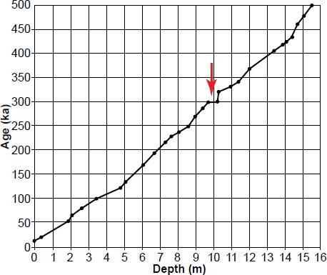
Fig. 4. Howard and Prell (1992) tuned age-depth model for the E49-18 sediment core. This tuned age-depth model required 28 chronological anchor points (the “dot” at 15.5 m was not an anchor point). Red arrow indicates an extremely shallow age versus depth slope, indicative of an extraordinarily high sedimentation rate.
Moreover, the tuned timescale of Howard and Prell (1992) required 28(!) chronological anchor points (see Fig. 4). This is remarkable, because one of the reasons Pacemaker seemed so convincing was because its results were obtained using simple age models only requiring a small number of anchor points. In the first part of the paper, for instance, results that were reasonably consistent with Milankovitch forcing were obtained using age models constructed from only two anchor points. Hence, the results were obtained without the need for extensive tuning of the timescale, seemingly an argument in favor of the Milankovitch hypothesis.
The fact that the tuned timescale for the entire E49-18 core required 28 anchor points suggests that the positive result for the E49-18 core presented in Pacemaker may have been a fluke. Obviously, a spectral analysis using 15.5 m worth of data is a much more stringent test of the Milankovitch hypothesis than a spectral analysis using only 10.6 m worth of data. The fact that a great deal of tuning was required when constructing an age model for the entire core raises an obvious question: what would be the results if one were to re-do the Pacemaker analysis, with the same procedure, but using all the data from the E49-18 core? Would the results still agree with Milankovitch expectations?
It should also be noted that Howard and Prell’s tuned age model is physically unrealistic (Fig. 5). If one numerically differentiates depth versus age, one sees that their model implies an outrageously high sedimentation rate of 50 cm/ka for 800 years, much higher than today’s global average of ~2 cm/ka (Vardiman 1996, 10). This does not bode well for attempts to re-do the Pacemaker analysis using all the data from the E49-18 core!
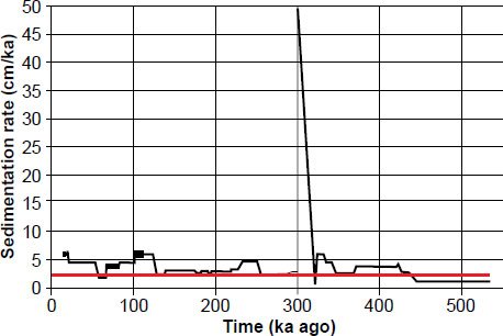
Fig. 5. Inferred sedimentation rate as a function of time for the E49-18 sediment core, based upon Howard and Prell’s tuned timescale and an assumption of no compression or disturbance of the sediments. Note the extremely high 50 cm/kyr sedimentation rate at ~300 ka. Although it is difficult to see from this graph, the “spike” lasts 800 years. For comparison, the horizontal red line marks 2 cm/ka, which is close to today’s worldwide marine average.
Pacemaker Problems: The Age of the Brunhes-Matuyama Magnetic Reversal Boundary
There is also a problem with the timescales that the Pacemaker authors assigned to E49-18 and RC11-120, especially the E49-18 core. Critical to these assigned timescales was an assumed age of 700,000 years for the most recent magnetic reversal boundary, the Brunhes-Matuyama (B-M) magnetic reversal boundary (Shackleton and Opdyke 1973, 40). Yet secular paleoclimatologists no longer accept this age as valid, having since revised the age of the B-M reversal upward to 780,000 years (Shackleton, Berger, and Peltier 1990). In fact, many now place the age as high as 790,000 years (Berger et al. 1995; Karner et al. 2002; Muller and MacDonald 2000, 159). If one were to reperform the original Pacemaker analysis, using the same technique to derive a timescale, but with the currently accepted age of 780 ka for the B-M magnetic reversal (rather than the old age of 700 ka), this would shift the ages of several of their chronological control or anchor points.
Constructing Timescales for the Two Cores: Chronological Anchor Points
Before performing spectral analysis on the two cores, the Pacemaker authors had to construct age depth models that would assign ages to the sediments. However, in order for their analysis to be a convincing confirmation of the Milankovitch hypothesis, these timescales needed to be independent of the Milankovitch hypothesis. Obviously, they could have simply tuned the sediment data in order to obtain a chronology that matched Milankovitch expectations, but doing so would have constituted circular reasoning. Hence, this process required a number of chronological control or anchor points, locations within the cores that had been dated by (presumably) independent means.
They first constructed a simple age model for each of the two cores, each of which used only two anchor points. They dubbed these their SIMPLEX age models. Having obtained (using the SIMPLEX age models) initial spectral results that were generally consistent with Milankovitch expectations, they then experimented with a more complicated model (which they dubbed ELBOW), as well as a tuned model, which they called TUNE-UP. They also constructed a composite data set called PATCH, which combined segments of data from the two cores. Three of these control points occurred at MIS boundaries. Four control points were determined for the RC11-120 core, and three were determined for E49-18.
They assigned an age of 0 ka to the top of RC11-120. As noted earlier, the second RC11-120 control point was an age of 9.4±0.6 ka assigned to a depth of 39 cm, on the basis of carbon-14 dating.
The B-M reversal boundary was used to assign the ages for the remaining control points. Shackleton and Opdyke (1973) had identified a complete magnetic reversal at a depth of 1200 cm in eastern Pacific core V28-238, a reversal which they concluded corresponded to the B-M reversal event. At the time, this reversal had been assigned an age of 700 ka (Shackleton and Opdyke 1973, 40). Assuming an age of 0 ka for the top of core V28-238 and, as a first approximation, a constant sedimentation rate for the upper 1200 cm of the core, Shackleton and Opdyke calculated an average sedimentation rate of 1200 cm ÷ 700 ka = 1.714 cm/ka. This assumed sedimentation rate was then used to assign ages to MIS boundaries within the V28-238 core. The Pacemaker authors then transferred these ages to the (presumed) corresponding MIS boundaries within the two Indian Ocean cores.
Within V28-238, the boundary between MIS 12 and 11 was located at a depth of 755 cm. The Pacemaker authors then used their assumed constant sedimentation rate (see Fig. 6) to assign an age of 755 cm ÷ 1.714 cm/ka = 440 ka to this MIS boundary (Shackleton and Opdyke 1973, 49). In a similar fashion, they assigned an age of 251 ka to the 8-7 boundary, which was located at a depth of 430 cm.
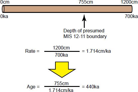
Fig. 6. Diagram illustrating the manner in which ages for marine isotope stage boundaries were estimated from the V28-238 sediment core.
This same technique yielded an age of 128 ka for the MIS 6-5 boundary (Shackleton and Opdyke 1973, 49). However, the Pacemaker authors opted to use a slightly lower estimate of 127 ka for this boundary when constructing their timescale (Hays, Imbrie, and Shackleton 1976, 1124). This estimated age of 127±6 ka was based upon 231Pa-230Th dating of Caribbean core V12-122 (Broecker and van Donk 1970, 173). No doubt the good agreement obtained from two different methods for this MIS boundary was seen as confirmation that the sedimentation rate within V28-238 was approximately constant.
Hays, Imbrie, and Shackleton (1976) then transferred these age assignments to the RC11-120 and E49-18 cores and obtained intermediate ages via interpolation in order to perform their analyses.
One may wonder why Shackleton and Opdyke (1973) chose the V28-238 core to estimate ages for MIS boundaries, given that hundreds of other cores had already been drilled. It should be remembered that by the early 1970s uniformitarian paleoclimatologists had already concluded that changes in sediment δ18O values were driven mainly by changes in global ice volume rather than by changes in temperature (Shackleton 1967; Wright 2010). Because the Pacific Ocean experiences smaller temperature fluctuations than does the Atlantic Ocean, they felt that a Pacific core, such as V28-238 would be a more suitable candidate for the development of an oxygen isotope stratigraphy than an Atlantic core. Likewise, they had concluded, on the basis of magnetic stratigraphy, that the equatorial Pacific region was a good candidate for particularly long sediment cores (Shackleton and Opdyke 1973, 39). They had also examined the nearby core V28-239, but noted that the top three meters of this core was severely disturbed (Shackleton and Opdyke 1973, 40). Hence, they did not feel it could be used. Thus, they viewed V28-238 as a good candidate for obtaining estimates for the ages of MIS stage boundaries.
The Effect of the New Age Estimate for the B-M Reversal Boundary
The fourth column in Table 1 contains the original age estimates for the three MIS boundaries used in Pacemaker (see Table 3 on p. 49 of Shackleton and Opdyke 1973, and Table 2 on p. 1124 in Pacemaker). These age estimates were based upon an assumed age of 700 ka for the B-M reversal boundary. The fifth column contains the new age estimates implied by an assumed age of 780 ka for this reversal boundary. One can easily verify these age estimates using simple arithmetic. This immediately results in a significant discordance between two different dating methods for the MIS 6-5 boundary: the age estimate of 127 ± 6 ka for the MIS 6-5 boundary (obtained via 231Pa-230Th dating of Caribbean core V12-122) and the age estimate of 143 ka (obtained by assuming a constant sedimentation rate in the V28-238 core). Hence, uniformitarian scientists must decide which of these two dates for the MIS 6-5 boundary is more trustworthy.
| MIS Boundary | Depth in V28-238 Core (cm) | Depth in E49-18 Core (cm) | Original Age Estimate BM Age of 700 ka | New Age Estimate BM Age of 780 ka |
|---|---|---|---|---|
| 6-5 | 220 | 490 | 128 | 143 |
| 8-7 | 430 | 825 | 251 | 280 |
| 12-11 | 755 | 1405 | 440 | 491 |
If they reject the estimate of 143 ka in favor of the 127 ka age, this means that the Pacemaker methodology used to assign ages to the 6-5, 8-7, and 12-11 MIS boundaries yields poor estimates for these boundaries when the new age estimate of 780 ka for the B-M reversal boundary is taken into account. This means that none of these three age estimates can really be trusted. And if that is the case, this means that any part of the Pacemaker analysis that used age estimates for the 8-7 and 12-11 boundaries is automatically suspect. This includes the analysis for the E49-18 core (both of its SIMPLEX age control points were tied to the age of the B-M reversal boundary), as well as the analysis of the PATCH “core,” which also depended upon these age control points. It also invalidates the test of statistical significance performed on the PATCH data set, as this data set also depended on age estimates for the 12-11 and 8-7 boundaries. This would leave Pacemaker without a valid test of statistical significance in the frequency domain, as this was the only such test performed in the paper.
On the other hand, if they reject the estimate of 127 ka for the MIS 6-5 boundary in favor of the 143 ka age assignment, this implies that the SIMPLEX timescales for the RC11-120 and E49-18 cores will be stretched. We illustrate this by considering the RC11-120 core. The original total time assigned to this core was 273 ka (see Table 3, p. 1124 in Pacemaker). Increasing the age of the MIS 6-5 boundary from 127 to 143 ka causes the total timescale to increase to 309 ka, as one can easily verify by assigning an age of 0 ka to the core top and an age of 143 ka to a depth of 4.40 m. Simple arithmetic and the assumption of a constant sedimentation rate implies an age of 309 ka for the core bottom. Hence, the timescale for the RC11-120 core will be stretched by about 13%. However, because the shapes of the climate signals within the cores are unaffected, one would expect the periods of the waves comprising those signals to also be stretched by 13%. This in turn means that the dominant peaks will also have periods that are about 13% larger than those originally reported in Pacemaker. Similar reasoning shows that the timescale for the bottom section of the E49-18 core would be stretched by about 11% (of course, these simple calculations are just ballpark estimates of the degree of stretching, as they ignore complications involved in the data analysis that might alter these new values). More important, this stretching of the timescales would introduce a very serious problem.
The Causality Problem Strikes Back
The reader may have already noticed that an age estimate of 143 ka for the MIS 6-5 (Termination II) boundary would imply that the penultimate deglaciation was occurring long before the solar insolation changes at about 130 ka ago that are supposed to have caused it. In other words, the Pacemaker paper, the primary argument for Milankovitch climate forcing, suffers from its own version of the causality problem! Hence, the argument from Pacemaker for Milankovitch climate forcing is equivocal. If uniformitarian scientists assume that the 127 ka age assignment for the MIS 6-5 boundary is correct, they can salvage the SIMPLEX results from the RC11-120 core, although these results may not be statistically significant. However, the spectral results from the E49-18 core and the PATCH “core” would be invalidated. On the other hand, if they accept the 143 ka age estimate as valid, the periods of the dominant spectral peaks will be stretched. Because some of the original calculated periods were already on the high side (two reported low-frequency peaks had periods as high as 119 and 122 ka), this stretching could cause some of these periods to be uncomfortably large. Worse yet, this would introduce a causality problem into Pacemaker. So no matter which option chosen by uniformitarian scientists, the paper, given the current accepted age for the B-M reversal, is not as strong as originally presented. Of course, if both age estimates are incorrect, as creation scientists would argue, then the paper is completely invalidated.
Some secular paleoclimatologists seem to have chosen the first option, as they still use an assigned age of ~127–130 ka for the MIS 6-5 boundary. For instance, the comprehensive stack of 57 global benthic δ18O records (Lisiecki and Raymo 2005, 7) assigns an age of 130 ka to the MIS 6-5 boundary (see the summary at http://www.lorraine-lisiecki.com/LR04_MISboundaries.txt, accessed 12/3/2015). However, some secular scientists might disagree, due to analysis of other data sets (Winograd et al. 1992).
Pacemaker Problems: “Evolving” Data Sets?
A third problem with Pacemaker is the fact that the data sets for the three climate variables used have “evolved” over time, making it hard to determine which data sets are the real ones. Multiple versions of the data can be found online, each subtly different from the other. In some cases, differences arise because researchers were only concerned with one section of the core and did not bother with values in other sections. Likewise, most of the differences in cited values are obviously attributable to minor measurement error. However, some of these differences are quite large, larger than the original cited analytical errors.
One possible reason for differences in the data sets is the phenomenon of sample heterogeneity (Barrows et al. 2007, 3). Because a given oxygen isotope ratio at a given depth is the average of measurements from many foraminiferal shells, inconsistency in these values can result if the sample size for a given depth is too small. One batch of foraminiferal shells at a given depth may yield one oxygen isotope ratio, while another batch from the same depth may yield another value that is outside the originally cited error bars.
Tables A1-A6 in the appendix show different versions of the RC11-120 and E49-18 data that I have found either online or have reconstructed from figures in published papers. The columns of data are in chronological order, with the oldest versions of the data on the left and the most recent versions on the right. I have included my reconstructed values of the data from the Pacemaker paper (discussed below), and these are graphically illustrated in Figs. 7–12. A side-by-side comparison of these different data versions is very revealing.
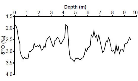
Fig. 7. My reconstructed RC11-120 planktonic δ18O values.
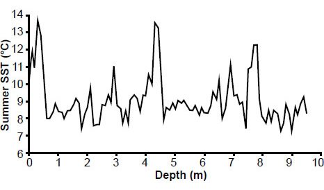
Fig. 8. Reconstructed RC11-120 summer sea surface temperature (SST) estimates.
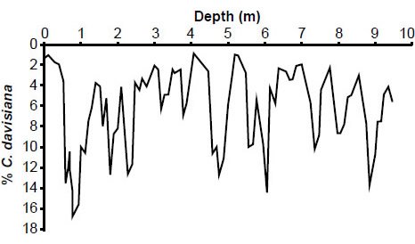
Fig. 9. Reconstructed RC11-120 % C. davisiana values.
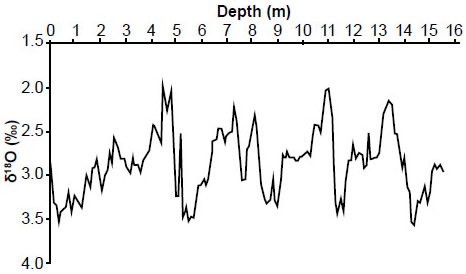
Fig. 10. Reconstructed E49-18 planktonic δ18O values. Data values above a depth of 3.5 meters were obtained from the column entitled “PANGAEA (1997)” in Table A2.
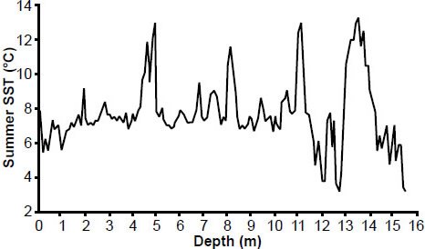
Fig. 11. Reconstructed E49-18 summer sea surface temperatures.
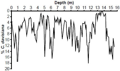
Fig. 12. Reconstructed E49-18 % C. davisiana values.
I now briefly discuss some of the variations in these data, using oxygen isotope values as an example. Table A1 in the appendix consists of oxygen isotope values for the RC11-120 core. The first three columns in the table, as well as the column labelled BM&H are values that I reconstructed from figures in papers, since I did not have access to these data in tabular form. There is an obvious discrepancy at the top of the core. Fig. 2 from Pacemaker indicates a δ18O value that is clearly much less than 2.0‰, (I estimated it to be 1.80‰) but Fig. 1 in Berger, Melice, and Hinnov (1991) indicates a δ18O value that is very close to 2.00 or 2.10‰.
Note also the anomalously high δ18O value of 20.31‰ at a depth of 0.80 m. Presumably this is a typo.
Also, data values are present in some versions of the data but are missing in later versions: note in particular the variations at depths of 5.70, 6.10, 8.70, and 8.90 m.
Some values have also been removed from later versions of the E49-18 δ18O data (Table A2 in the appendix): note especially the changes at depths of 3.70, 9.10, 13.80, 14.80, and 15.50 m.
Perhaps the most dramatic difference is seen in the (southern hemisphere) summer sea surface temperature (SST) estimates for the E49-18 core. Examination of Table A4 in the appendix shows that (Howard and Prell 1992) obtained their own SST estimates based on foraminiferal data within the core (Fig. 13). Although these new temperature variations are generally in phase with the original temperature estimates (based upon radiolarian data), they are generally of lesser amplitude. This raises the question: which of these two data sets should be used in a spectral analysis? Which data set provides better estimates of summer sea surface temperatures?
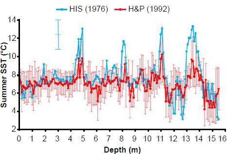
Fig. 13. Original Pacemaker (HIS) southern hemisphere summer sea surface temperature estimates (in blue), based upon radiolarian data within the E49-18 sediment core, and later estimates (in red) by Howard and Prell (1992), based upon foraminiferal data. The uncertainty in the original estimates (blue error bars) were estimated by HIS to be ±1.5°C. Red error bars indicate error estimates by Howard and Prell (see appendix for details).
Variations in other quantities are seen in the other tables.
In spite of the fact that different versions of the data sometimes exist, I have been unable to find the original, unaltered 10 cm resolution data used in the Pacemaker paper, and repeated requests for these data to the two surviving Pacemaker authors (Hays and Imbrie) went unanswered. However, I was able to reconstruct these data from Figs. 2 and 3 in Pacemaker (a tedious process, to be sure). It should be noted that in some cases my reconstructed values have been reported to the third decimal place: this was necessary in order to obtain a good visual fit to the published figures, and I felt that this was more important than slavish adherence to significant figure rules. Although I do not have legal permission to reproduce Figs. 2 and 3 from the Pacemaker authors (this request also went unanswered), reproductions of these two figures are ubiquitous on the internet, and one can easily verify that there is a good visual match between my Figs. 7–12 and the graphs from the Pacemaker paper.
Summary and Conclusion
Although Pacemaker is widely seen as having confirmed the Milankovitch hypothesis of Pleistocene ice ages, it is characterized by at least three serious problems. First, a large section of the E49-18 data may have been needlessly excluded from the analysis. Second, before the paper’s authors could obtain power spectra for the climatic variables within the two cores, they had to construct chronologies for the two cores. The ages for two of the marine isotope stages which served as chronological anchor points were directly tied to the presumed age of 700,000 years for the Brunhes-Matuyama magnetic reversal, an age which is significantly younger than the currently accepted age of 780,000–790,000 years. This age revision weakens the paper, either by invalidating a large part of the analysis, and/or by introducing a causality problem into the results. Third, multiple versions of the same data exist, each a little different from each other. Why do these data sets keep changing?
Finally, it should be noted that the method the authors used to assign ages to the MIS 6-5, 8-7, and 12-11 boundaries is inherently risky, even within a uniformitarian framework. Given that free-floating planktonic foraminifera are more likely than benthic foraminifera to experience short-term variations in temperature due to local effects, and given that the authors made no attempt to remove the effect of local “noise,” how can they be sure these oxygen isotope values are truly indicative of a globally synchronous signal? The manner in which they transferred ages from the V28-238 and V12-122 cores to the RC11-120 and E49-18 cores was based on little more than an apparent visual match between the different oxygen isotope signals.
Part II of this series continues this discussion, with an explanation of the technical details of the Pacemaker analysis and partial replication of the original results. Part III explores the effect that the above changes in timescale have on the original results, as well as the implications for geochronology and the debate over global warming/climate change.
References
Austin, S. A. 1994. “Interpreting Strata of Grand Canyon.” In Grand Canyon: Monument to Catastrophe. Edited by S. A. Austin, 21–56. Santee, California: Institute for Creation Research.
Barrows, T. T., S. Juggins, P. De Deckker, E. Calvo, and C. Pelejero. 2007. “Long-Term Sea Surface Temperature and Climate Change in the Australian-New Zealand Region.” Paleoceanography 22 (2). (PA2215).
Berger, W. H., T. Bickert, G. Wefer, and M. K. Yasuda. 1995. “Brunhes-Matuyama Boundary: 790 k.y. Date Consistent with ODP Leg 130 Oxygen Isotope Records Based on Fit to Milankovitch Template.” Geophysical Research Letters 22 (12): 1525–28.
Berger, A., JL. Melice, and L. Hinnov. 1991. “A Strategy for Frequency Spectra of Quaternary Climate Records.” Climate Dynamics 5 (4): 227–40.
Blaauw, M. 2010. “Out of Tune: The Dangers of Aligning Proxy Archives.” Quaternary Science Reviews 36: 38–49.
Blaauw, M., K. D. Bennett, and J. A. Christen. 2010. “Random Walk Simulations of Fossil Proxy Data.” The Holocene 20 (4): 645–49.
Boyle, E. A., and L. D. Keigwin. 1985. “Comparison of Atlantic and Pacific Paleochemical Records for the Last 215,000 Years: Changes in Deep Ocean Circulation and Chemical Inventories.” Earth and Planetary Science Letters 76 (1–2): 135–50.
Broecker, W. S., and G. M. Henderson. 1998. “The Sequence of Events Surrounding Termination II and their Implications for the Cause of Glacial-Interglacial CO2 Changes.” Paleoceanography 13 (4): 352–64.
Broecker, W. S., and J. van Donk. 1970. “Insolation Changes, Ice Volumes, and the O18 Record in Deep-Sea Cores.” Reviews of Geophysics and Space Physics 8 (1): 169–98.
Cande, S. C., and D. V. Kent. 1992. “A New Geomagnetic Polarity Time Scale for the Late Cretaceous and Cenozoic.” Journal of Geophysical Research 97 (B10): 13917–51.
Cheng, H., R. L. Edwards, M. T. Murrell, and T. M. Benjamin. 1998. “Uranium-Thorium-Protactinium Dating Systematics.” Geochimica et Cosmochimica Acta 62 (21–22): 3437–52.
CLIMAP Project Members. 1981. “Seasonal Reconstruction of the Earth’s Surface at the Last Glacial Maximum.” Map and Chart Series 36: 1–18. Geological Society of America.
Corliss, B. H., and R. C. Thunell. 1983a. “Carbonate Sedimentation Beneath the Antarctic Circumpolar Current during the late Quaternary.” Marine Geology 51 (3–4): 293–326.
Corliss, B. H., and R. C. Thunell. 1983b. “Carbonate Sedimentation Beneath the Antarctic Circumpolar Current.” Antarctic Journal of the United States 18(5): 141–42.
Cronin, T. M. 2010. Paleoclimates: Understanding Climate Change Past and Present. New York, New York: Columbia University Press.
Dietrich, T. K. 2011. The Culture of Astronomy: Origin of Number, Geometry, Science, Law, and Religion. Minneapolis, Minnesota: Beacon Hill Publishing Group.
Emiliani, C. 1966. “Isotopic Paleotemperatures.” Science 154 (3751): 851–57.
Epstein, S., R. Buchsbaum, H. A. Lowenstam, and H. C. Urey. 1953. “Revised Carbonate-Water Isotopic Temperature Scale.” Bulletin of the Geological Society of America 64 (11): 1315–26.
Frakes, L. A. 1973. USNS Eltanin Sediment Descriptions: Cruises 4-54. Contribution (Florida State University, Sedimentological Research Laboratory) no. 37. Tallahassee, Florida: Florida State University.
Gibbard, P. L. 2007. “Climatostratigraphy.” In Encyclopedia of Quaternary Science. Edited by S. A. Elias, 2819–25. Amsterdam, The Netherlands: Amsterdam. Quoted in modified form by the INQUA Commission on Stratigraphy and Chronology. http://www.inqua-saccom.org/stratigraphic-guide/climatostratigraphy-geological-climate-stratigraphy/.
Hays, J. D. 1997. “Sea Surface Temperature Reconstruction from Sediment Core RC11-120 (specmap.051).” doi:10.1594/PANGAEA.52223.
Hays, J. D., J. Imbrie, and N. J. Shackleton. 1976. “Variations in the Earth’s Orbit: Pacemaker of the Ice Ages.” Science 194 (4270): 1121–132.
Hays, J. D., J. D. Imbrie, and N. J. Shackleton. 1997. “Stable Isotopes of Sediment Core ELT49.018-PC (specmap2.006).” doi:10.1594/PANGAEA.52207.
Hays, J. D., J. A. Lozano, N. Shackleton, and G. Irving. 1976. “Reconstruction of the Atlantic and Western Indian Ocean Sectors of the 18,000 B.P. Antarctic Ocean.” Geological Society of America Memoir 145: 337–72.
Hebert, J. 2014. “Circular Reasoning in the Dating of Deep Seafloor Sediments and Ice Cores: The Orbital Tuning Method.” Answers Research Journal 7: 297–309, https://answersingenesis.org/age-of-the-earth/circular-reasoning-dating-deep-seafloor-sediments-and-ice-cores-orbital-tuning-method/.
Hebert, J. 2015. “The Dating ‘Pedigree’ of Seafloor Sediment Core MD97-2120: A Case Study.” Creation Research Society Quarterly 51 (3): 152–64.
Herbert, T. D. 2010. “Paleoceanography: Orbitally Tuned Timescales.” In Climates and Oceans, 370–77. Editor-in-chief J. H. Steele. Amsterdam, The Netherlands: Academic Press.
Hinnov, L. A., and F. J. Hilgen. 2012. “Cyclostratigraphy and Astrochronology.” In The Geologic Time Scale 2012. Edited by F. M. Gradstein, J. G. Ogg, M. D. Schmitz, and G. M. Ogg, 63–83. Amsterdam, The Netherlands: Elsevier.
Howard, W. R., and W. L. Prell. 1992. “Late Quaternary Surface Circulation of the Southern Indian Ocean and Its Relationship to Orbital Variations.” Paleoceanography 7 (1): 79–117.
Imbrie, J. 1982. “Astronomical Theory of the Pleistocene Ice Ages: A Brief Historical Review.” Icarus 50 (2–3): 408–22.
Karner, D. B., and R. A. Muller. 2000. “A Causality Problem for Milankovitch.” Science 288 (5474): 2143–44.
Karner, D. B., J. Levine, B. P. Medeiros, and R. A. Muller. 2002. “Constructing a Stacked Benthic δ18O Record.” Paleoceanography 17 (3): 2-1-2-16.
Kingston, P. F. 2010. “Benthic Organisms Overview.” In Climates and Oceans. Editor-in-chief J. H. Steele, 416–24. Amsterdam, The Netherlands: Academic Press.
Lisiecki, L. E., and M. E. Raymo. 2005. “A Pliocene-Pleistocene Stack of 57 Globally Distributed Benthic δ18O Records.” Paleoceanography 20 (1): PA1003.
Martinson, D. G., N. G. Pisias, J. D. Hayes, J. Imbrie, T. C. Moore, and N. J. Shackleton. 1987. “Age Dating and the Orbital Theory of the Ice Ages: Development of a High-Resolution 0 to 300,000-year Chronostratigraphy.” Quaternary Research 27 (1): 1–29.
McDuff, R. E., and G. R. Heath. 2001. Proxies: Oceanic Records of Pleistocene Climatic Change. http://www2.ocean.washington.edu/oc540/lec01-24/.
McIntyre, A., and J. D. Imbrie. 2000. “Stable Isotope of Sediment Core RC11-120 (specmap.013).” doi:10.1594/PANGAEA.56357.
Milanković, M. 1941. Kanon der Erdbestrahlung und seine Anwendung auf das E iszeitenproblem (Canon of Insolation and the Ice-Age Problem). Belgrade, Serbia: Special Publications of the Royal Serbian Academy. Vol. 132.
Mix, A. C., and R. G. Fairbanks. 1985. “North Atlantic Surface-Ocean Control of Pleistocene Deep-Ocean Circulation.” Earth and Planetary Science Letters 73 (2–4): 231–43.
Mortyn, P. G., and C. D. Charles. 2003. “Planktonic Foraminiferal Depth Habitat and δ18O Calibrations: Plankton Tow Results from the Atlantic Sector of the Southern Ocean.” Paleoceanography 18 (2): 1037.
Muller, R. A., and G. J. MacDonald. 1997. “Spectrum of 100-kyr Glacial Cycle: Orbital Inclination, not Eccentricity.” Proceedings of the National Academy of Sciences 94 (16): 8329–34.
Muller, R. A., and G. J. MacDonald. 2000. Ice Ages and Astronomical Causes: Data, Spectral Analysis and Mechanisms. Chichester, United Kingdom: Praxis Publishing.
Neeman, B. U. 1993. “Orbital Tuning of Paleoclimatic Records: A Reassessment.” Lawrence Berkeley National Laboratory Report LBNL-39572.
Oard, M. J. 1984. “Ice Ages: The Mystery Solved? Part II: The Manipulation of Deep-Sea Cores.” Creation Research Society Quarterly 21 (3): 125–37.
Oard, M. J. 2000. “How Well Do Paleontologists Know Fossil Distributions?” Creation Ex Nihilo Technical Journal 14 (1): 7–8.
Oard, M. J. 2007. “Astronomical Troubles for the Astronomical Hypothesis of Ice Ages.” Journal of Creation 21 (3): 19–23.
Oard, M. J. 2010. “Further Expansion of Evolutionary Fossil Time Ranges.” Journal of Creation 24 (3): 5–7.
Patrick, K. 2010. “Manganese Nodules and the Age of the Ocean Floor.” Journal of Creation 24 (3): 82–86.
Raymo, M. E. 1992. “Global Climate Change: A Three Million Year Perspective.” Start of a Glacial, Proceedings of the Mallorca NATO ARW, NATO ASI Series I. Vol. 3. Edited by G. Kukla and E. Went, 207–23. Heidelberg, Germany: Springer-Verlag.
Raymo, M. E., W. F. Ruddiman, J. Backman, B. M. Clement, and D. G. Martinson. 1989. “Late Pliocene Variation in Northern Hemisphere Ice Sheets and North Atlantic Deep Circulation.” Paleoceanography 4 (4): 413–46.
Rickaby, R. E. M., and H. Elderfield. 1999. “Planktonic Foraminiferal Cd/Ca: Paleonutrients or Paleotemperature?” Paleoceanography 14(3): 293–303.
Ruddiman, W. F., M. E. Raymo, D. G. Martinson, B. M. Clement, and J. Backman. 1989. “Pleistocene Evolution of Northern Hemisphere Climate. Paleoceanography 4 (4): 353–412.
Shackleton, N. 1967. “Oxygen Isotope Analyses and Pleistocene Temperatures Re-assessed.” Nature 215 (5096): 15–17.
Shackleton, N. J., A. Berger, and W. R. Peltier. 1990. “An Alternative Astronomical Calibration of the Lower Pleistocene Timescale Based on ODP Site 677.” Transactions of the Royal Society of Edinburgh: Earth Sciences 81 (4): 251–61.
Shackleton, N. J. and N. D. Opdyke. 1973. “Oxygen Isotope and Palaeomagnetic Stratigraphy of Equatorial Pacific Core V28-238: Oxygen Isotope Temperatures and Ice Volumes on a 105 and 106 Year Scale.” Quaternary Research 3 (1): 39–55.
Shakun, J. D., S. J. Burns, P. U. Clark, H. Cheng, and R. L. Edwards. 2011. “Milankovitch-paced Termination II in a Nevada Speleothem?” Geophysical Research Letters 38 (18): L18701.
Siddall, M., E. Bard, E. J. Rohling, and C. Hemleben. 2006. “Sea-Level Reversal during Termination II.” Geology 34 (10): 817–20.
Stanley, G. D., Jr. 1998. “A Triassic Sponge from Vancouver Island: Possible Holdover from the Cambrian.” Canadian Journal of Earth Sciences 35 (9): 1037–43.
Vardiman, L. 1996. Sea-Floor Sediment and the Age of the Earth. El Cajon, California: Institute for Creation Research.
Walker, M., and J. Lowe. 2007. “Quaternary Science 2007: A 50-year Retrospective.” Journal of the Geological Society 164 (6): 1073–92.
Winograd, I. J., T. B. Coplen, J. M. Landwehr, A. C. Riggs, K. R. Ludwig, B. J. Szabo, P. T. Kolesar, and K. M. Revesz. 1992. “Continuous 500,000-Year Climate Record from Vein Calcite in Devils Hole, Nevada.” Science 258 (5080): 255–260.
Wolff, E. W., J. Chappellaz, T. Blunier, S. O. Rasmussen, and A. Svensson. 2010. “Millennial-Scale Variability during the Last Glacial: The Ice Core Record.” Quaternary Science Reviews 29 (21-22): 2828–38.
Wright, J. D. 2010. “Cenozoic Climate—Oxygen Isotope Evidence.” In Climates and Oceans. Editor-in-chief J. H. Steele, 316–27. Amsterdam, The Netherlands: Academic Press.
Appendix
Data from Sediment Cores RC11-120 and E49-18
Tables A1-A6 contain different versions of the data sets from sediment cores RC11-120 and E49-18. Tables A1 and A2 contain oxygen isotope data obtained from the planktonic foram Globigerina bulloides (using the Peedee belemnite standard). Tables A3 and A4 contain (southern hemisphere) summer sea surface temperature estimates (°C), based upon interpretation of radiolarian data within the cores. Tables A5 and A6 contain the relative abundance of one particular radiolarian species, Cycladophora davisiana, expressed as a percentage. The keys below provide the references for the values in the six tables. The original “pacemaker” paper is the only source that I could find for C. davisiana data for the E49-18 core. In some cases, multiple values are cited within a single data set , and these multiple values are reported, separated by commas.
| Depth (m) | HLS&I (Fig. 3) | HLS&I (Fig. 4) | HI&S | C-long | C-short | S-Martinson | BM&H | R&E | S-M&I |
|---|---|---|---|---|---|---|---|---|---|
| 0.00 | 1.80 | 2.10 | |||||||
| 0.025 | 2.06 | ||||||||
| 0.05 | 1.92, 1.96 | 2.06 | 1.84,1.99,2.27 | 1.87 | 1.88 | 1.87 | |||
| 0.10 | 1.91 | 1.90 | 1.91 | 1.96 | 1.913 | 1.96 | 1.96 | ||
| 0.12 | 2.07 | ||||||||
| 0.15 | 1.9 | 1.97 | 1.900 | 1.965 | 1.97 | ||||
| 0.20 | 2.03 | 2.10 | 2.00 | 2.15 | 1.96 | 2.013 | 1.96 | 1.96 | |
| 0.25 | 2.03 | 2.04 | 2.16 | 2.150 | 2.11 | 2.16 | |||
| 0.30 | 2.34 | 2.40 | 2.33, 2.37 | 2.38 | 2.013 | 2.38 | 2.38 | ||
| 0.35 | 2.18 | 2.13, 2.2 | 2.32 | 2.350 | 2.3 | 2.32 | |||
| 0.40 | 2.59 | 2.70 | 2.55 | 2.55, 2.67 | 2.60 | 2.175 | 2.59 | 2.60 | |
| 0.45 | 2.74 | 2.74 | 2.74 | 2.700 | 2.74 | 2.74 | |||
| 0.50 | 3.01 | 3.12 | 3.01 | 2.98 | 3.000 | 2.98 | 2.98 | ||
| 0.55 | 2.91 | 2.92 | 2.95 | 2.913 | 2.95 | 2.95 | |||
| 0.60 | 3.24 | 3.40 | 3.24 | 3.33 | 3.37 | 3.350 | 3.37 | 3.37 | |
| 0.65 | 3.28 | 3.28 | 3.28 | ||||||
| 0.70 | 3.34 | 3.33 | 3.34 | 3.53 | 3.363 | 3.475 | 3.53 | ||
| 0.75 | 3.34 | 3.37 | 3.34 | ||||||
| 0.80 | 3.18 | 3.35 | 3.23 | 3.29, 20.31 | 3.36 | 3.288 | 3.33 | 3.36 | |
| 0.85 | 3.43 | 3.45 | 3.43 | ||||||
| 0.90 | 3.32 | 3.31 | 3.32 | 3.34 | 3.325 | 3.34 | 3.34 | ||
| 0.95 | 3.31 | 3.31 | 3.31 | ||||||
| 1.00 | 3.33 | 3.41 | 3.30 | 3.32 | 3.29 | 3.325 | 3.35 | 3.29 | |
| 1.05 | 3.32 | 3.32 | 3.32 | ||||||
| 1.10 | 3.31 | 3.29 | 3.30 | 3.22 | 3.300 | 3.22 | 3.22 | ||
| 1.15 | 3.07 | 3.07 | 3.07 | ||||||
| 1.20 | 3.01 | 3.10 | 3.00 | 3.01 | 3.04 | 3.000 | 3.04 | 3.04 | |
| 1.25 | 3.07 | 3.1 | 3.07 | ||||||
| 1.30 | 3.04 | 3.00 | 3.03 | 2.96 | 3.013 | 3.19 | 3.19 | ||
| 1.35 | 2.96 | 2.95 | 2.96 | ||||||
| 1.40 | 2.92 | 3.00 | 2.93 | 2.92 | 3.11 | 2.900 | 3.1 | 3.11 | |
| 1.45 | 2.98 | 2.98 | 2.98 | ||||||
| 1.50 | 2.87 | 2.90 | 2.88 | 3.05 | 2.875 | 3.05 | 3.05 | ||
| 1.55 | 2.70 | 2.69 | 3.01 | 2.700 | 3.07 | 3.01 | |||
| 1.60 | 2.65 | 2.65 | 2.61, 2.7 | 2.94 | 2.650 | 2.94 | 2.94 | ||
| 1.65 | 2.81 | 2.80 | 2.98 | 2.788 | 2.98 | 2.98 | |||
| 1.70 | 2.83 | 2.80 | 2.81 | 2.95 | 2.794 | 2.96 | 2.95 | ||
| 1.75 | 2.82 | 2.81 | 2.89 | 2.800 | 2.9 | 2.89 | |||
| 1.80 | 2.73 | 2.80 | 2.74 | 2.90 | 2.750 | 2.92 | 2.90 | ||
| 1.85 | 2.99 | 2.99 | 2.66 | 2.988 | 2.66 | 2.66 | |||
| 1.90 | 2.76 | 2.75 | 2.75 | 2.86 | 2.750 | 2.89 | 2.86 | ||
| 1.95 | 2.88 | 2.87 | 2.87 | 2.863 | 2.92 | 2.87 | |||
| 2.00 | 2.86 | 2.80 | 2.86 | 2.82 | 2.863 | 2.82 | 2.82 | ||
| 2.05 | 2.82 | 2.8 | 2.82 | ||||||
| 2.10 | 2.70 | 2.70 | 2.72 | 3.03 | 2.725 | 3.04 | 3.03 | ||
| 2.15 | 2.76 | 2.8 | 2.76 | ||||||
| 2.20 | 2.94 | 2.95 | 2.94 | 3.08 | 2.925 | 3.16 | 3.08 | ||
| 2.25 | 3.15 | 3.18 | 3.15 | ||||||
| 2.30 | 2.92 | 2.90 | 2.93 | 2.84 | 2.900 | 2.79 | 2.84 | ||
| 2.35 | 2.98 | 3.04 | 2.98 | ||||||
| 2.40 | 2.78 | 2.75 | 2.77 | 2.85 | 2.775 | 2.85 | 2.85 | ||
| 2.45 | 2.82 | 2.82 | 2.82 | ||||||
| 2.50 | 2.86 | 2.85 | 2.85 | 2.71 | 2.850 | 2.71 | 2.71 | ||
| 2.55 | 2.59 | 2.59 | 2.59 | ||||||
| 2.60 | 2.54 | 2.55 | 2.54 | 2.54 | 2.538 | 2.53 | 2.54 | ||
| 2.65 | 2.55 | 2.51 | 2.55 | ||||||
| 2.70 | 2.50 | 2.45 | 2.50 | 2.59 | 2.500 | 2.59 | 2.59 | ||
| 2.75 | 2.44 | 2.44 | 2.44 | ||||||
| 2.80 | 2.38 | 2.38 | 2.38 | 2.43 | 2.400 | 2.47 | 2.43 | ||
| 2.85 | 2.42 | 2.42 | 2.42 | ||||||
| 2.90 | 2.35 | 2.35 | 2.35 | 2.37 | 2.350 | 2.37 | 2.37 | ||
| 2.95 | 2.40 | 2.4 | 2.40 | ||||||
| 3.00 | 2.58 | 2.60 | 2.56 | 2.71 | 2.500 | 2.71 | 2.71 | ||
| 3.05 | 2.61 | 2.61 | 2.61 | ||||||
| 3.10 | 2.74 | 2.75 | 2.72 | 2.68 | 2.600 | 2.62 | 2.68 | ||
| 3.15 | 2.58 | 2.58 | 2.58 | ||||||
| 3.20 | 2.82 | 2.8 | 2.81 | 2.68 | 2.788 | 2.68 | 2.68 | ||
| 3.25 | 2.54 | 2.6 | 2.54 | ||||||
| 3.30 | 2.50 | 2.52 | 2.50 | 2.60 | 2.500 | 2.6 | 2.60 | ||
| 3.35 | 2.40 | 2.4 | 2.40 | ||||||
| 3.40 | 2.48 | 2.50 | 2.49 | 2.54 | 2.488 | 2.53 | 2.54 | ||
| 3.45 | 2.48 | 2.47 | 2.48 | ||||||
| 3.50 | 2.39 | 2.40 | 2.41 | 2.42 | 2.425 | 2.45 | 2.42 | ||
| 3.55 | 2.40 | 2.4 | 2.40 | ||||||
| 3.60 | 2.43 | 2.43 | 2.44 | 2.48 | 2.450 | 2.52 | 2.48 | ||
| 3.65 | 2.45 | 2.45 | 2.45 | ||||||
| 3.70 | 2.55 | 2.60 | 2.58 | 2.48 | 2.575 | 2.48 | 2.48 | ||
| 3.75 | 2.46 | 2.46 | 2.46 | ||||||
| 3.80 | 2.65 | 2.70 | 2.65 | 2.72, 2.52, 2.63 | 2.62 | 2.650 | 2.62 | 2.62 | |
| 3.85 | 2.48, 2.52 | 2.50 | 2.48 | 2.50 | |||||
| 3.90 | 2.70 | 2.60 | 2.70 | 2.65, 2.56 | 2.61 | 2.675 | 2.61 | 2.61 | |
| 3.95 | 2.38, 2.46 | 2.42 | 2.42 | 2.42 | |||||
| 4.00 | 2.53 | 2.50 | 2.52 | 2.43, 2.24, 2.32 | 2.33 | 2.575 | 2.34 | 2.33 | |
| 4.05 | 2.15, 2.12 | 2.14 | 2.14 | 2.14 | |||||
| 4.10 | 2.40 | 2.40 | 2.39 | 2.20, 2.26 | 2.23 | 2.400 | 2.23 | 2.23 | |
| 4.15 | 1.88, 1.77 | 1.83 | 1.83 | 1.83 | |||||
| 4.20 | 1.85 | 1.84 | 1.72, 1.79, 2 | 1.88, 1.89 | 1.89 | 1.863 | 1.88 | 1.89 | |
| 4.25 | 1.80, 1.78, 1.79 | 1.79 | 1.89 | 1.79 | |||||
| 4.30 | 1.94 | 1.92 | 1.94 | 1.91, 1.90 | 1.91 | 1.925 | 1.91 | 1.91 | |
| 4.35 | 2.06, 2.51, 2.47 | 2.35 | 2.28 | 2.35 | |||||
| 4.40 | 2.62 | 2.55 | 2.5, 2.71 | 2.69, 2.68, 2.78 | 2.72 | 2.488 | 2.68 | 2.72 | |
| 4.45 | 2.79, 2.85 | 2.82 | 2.81 | 2.82 | |||||
| 4.50 | 3.12 | 3.12 | 3.13 | 3.14, 3.34, 3.05 | 3.18 | 3.050 | 3.24 | 3.18 | |
| 4.55 | 3.03, 3.26, 3.31 | 3.20 | 3.15 | 3.20 | |||||
| 4.60 | 3.31 | 3.30 | 3.31 | 3.53, 3.34, 3.46 | 3.44 | 3.300 | 3.44 | 3.44 | |
| 4.65 | 3.28, 3.34 | 3.31 | 3.313 | 3.31 | |||||
| 4.70 | 3.33 | 3.33 | 3.52, 3.56 | 3.54 | 3.313 | 3.52 | 3.54 | ||
| 4.75 | 3.34, 3.02 | 3.18 | 3.18 | 3.18 | |||||
| 4.80 | 3.38 | 3.38 | 3.37 | 3.32, 3.42 | 3.37 | 3.363 | 3.27 | 3.37 | |
| 4.85 | 3.42 | 3.42 | 3.42 | ||||||
| 4.90 | 3.45 | 3.42 | 3.10 | 3.413 | 3.10 | ||||
| 4.95 | 3.14 | 3.14 | |||||||
| 5.00 | 3.27 | 3.23 | 3.38 | 3.250 | 3.38 | ||||
| 5.05 | 3.25 | 3.25 | |||||||
| 5.10 | 3.32 | 3.32 | 3.19 | 3.300 | 3.19 | ||||
| 5.15 | 3.27 | 3.27 | |||||||
| 5.20 | 3.27 | 3.24 | 3.21 | 3.250 | 3.21 | ||||
| 5.25 | 3.22 | 3.22 | |||||||
| 5.30 | 3.36 | 3.35 | 3.24 | 3.288 | 3.24 | ||||
| 5.35 | 3.27 | 3.27 | |||||||
| 5.40 | 3.35 | 3.35 | 3.21 | 3.325 | 3.21 | ||||
| 5.45 | 3.15 | 3.15 | |||||||
| 5.50 | 3.30 | 3.33 | 3.32 | 3.288 | 3.32 | ||||
| 5.55 | 3.15 | 3.15 | |||||||
| 5.60 | 3.27 | 3.24 | 3.21 | 3.250 | 3.21 | ||||
| 5.65 | 3.13 | 3.13 | |||||||
| 5.70 | 3.15 | 3.06 | 3.050 | 3.06 | |||||
| 5.75 | 2.90 | 2.90 | |||||||
| 5.80 | 2.90 | 2.85 | 2.91 | 2.850 | 2.91 | ||||
| 5.85 | 2.87 | 2.87 | |||||||
| 5.90 | 3.00 | 3.01 | 2.81 | 3.000 | 2.81 | ||||
| 5.95 | 2.81 | 2.81 | |||||||
| 6.00 | 2.85 | 2.88 | 3.02 | 2.875 | 3.02 | ||||
| 6.05 | 2.85 | 2.85 | |||||||
| 6.10 | 2.83 | 2.82 | 2.78 | 2.825 | |||||
| 6.15 | 2.61 | 2.61 | |||||||
| 6.20 | 2.70 | 2.67 | 2.59 | 2.563 | 2.59 | ||||
| 6.25 | 2.55 | 2.55 | |||||||
| 6.30 | 2.29 | 2.31 | 2.43 | 2.325 | 2.43 | ||||
| 6.35 | 2.32 | 2.32 | |||||||
| 6.40 | 2.40 | 2.38 | 2.18 | 2.388 | 2.18 | ||||
| 6.45 | 2.17 | 2.17 | |||||||
| 6.50 | 2.10 | 2.11 | 2.14 | 2.125 | 2.14 | ||||
| 6.55 | 2.41 | 2.41 | |||||||
| 6.60 | 2.40 | 2.38 | 2.52 | 2.375 | 2.52 | ||||
| 6.65 | 2.49 | 2.49 | |||||||
| 6.70 | 2.30 | 2.35 | 2.45 | 2.363 | 2.45 | ||||
| 6.75 | 2.13 | 2.13 | |||||||
| 6.80 | 2.55 | 2.53 | 2.31 | 2.513 | 2.31 | ||||
| 6.85 | 2.24 | 2.24 | |||||||
| 6.90 | 2.28 | 2.28 | 2.20 | 2.275 | 2.20 | ||||
| 6.95 | 2.47 | 2.47 | |||||||
| 7.00 | 2.50 | 2.5 | 2.70 | 2.425 | 2.70 | ||||
| 7.05 | 2.55 | 2.55 | |||||||
| 7.10 | 2.80 | 2.81 | 2.62 | 2.719 | 2.62 | ||||
| 7.15 | 2.62 | 2.62 | |||||||
| 7.20 | 3.05 | 3.04 | 2.86 | 3.013 | 2.86 | ||||
| 7.25 | 2.85 | 2.85 | |||||||
| 7.30 | 3.00 | 3 | 2.72 | 2.988 | 2.72 | ||||
| 7.35 | 2.74 | 2.74 | |||||||
| 7.40 | 2.80 | 2.80 | 2.78 | 2.769 | 2.78 | ||||
| 7.45 | 2.46 | 2.46 | |||||||
| 7.50 | 2.55 | 2.54 | 2.46 | 2.550 | 2.46 | ||||
| 7.55 | 2.45 | 2.45 | |||||||
| 7.60 | 2.60 | 2.62 | 2.57 | 2.600 | 2.57 | ||||
| 7.65 | 2.38 | 2.38 | |||||||
| 7.70 | 2.40 | 2.38 | 2.39 | 2.400 | 2.39 | ||||
| 7.75 | 2.62 | 2.62 | |||||||
| 7.80 | 2.55 | 2.55 | 2.71 | 2.575 | 2.71 | ||||
| 7.85 | 2.67 | 2.67 | |||||||
| 7.90 | 2.95 | 2.94 | 2.86 | 2.925 | 2.86 | ||||
| 7.95 | 3.03 | 3.03 | |||||||
| 8.00 | 3.00 | 2.98 | 2.92 | 2.950 | 2.92 | ||||
| 8.05 | 2.99 | 2.99 | |||||||
| 8.10 | 2.95 | 2.93 | 2.94 | 2.925 | 2.94 | ||||
| 8.15 | 3.05 | ||||||||
| 8.20 | 3.11 | 3.11 | 2.97 | 3.113 | 2.97 | ||||
| 8.25 | 2.88 | 2.88 | |||||||
| 8.30 | 2.70 | 2.7 | 2.84 | 2.700 | 2.84 | ||||
| 8.35 | 2.91 | 2.91 | |||||||
| 8.40 | 3.00 | 3.05 | 3.04 | 3.025 | 3.04 | ||||
| 8.45 | 2.94 | 2.94 | |||||||
| 8.50 | 2.80 | 2.81 | 2.85 | 2.800 | 2.85 | ||||
| 8.55 | 2.95 | 2.95 | |||||||
| 8.60 | 3.09 | 3.15 | 3.15 | 3.138 | |||||
| 8.65 | 2.43 | ||||||||
| 8.70 | 2.90 | 3.019 | |||||||
| 8.75 | |||||||||
| 8.80 | 2.90 | 2.91 | 2.91 | 2.900 | |||||
| 8.85 | |||||||||
| 8.90 | 3.00 | 3 | 3.00 | 3.000 | |||||
| 8.95 | 2.91 | 2.91 | |||||||
| 9.00 | 2.70 | 2.74 | 2.79 | 2.763 | 2.79 | ||||
| 9.05 | 2.80 | 2.80 | |||||||
| 9.10 | 2.65 | 2.64 | 2.58 | 2.625 | 2.58 | ||||
| 9.15 | 2.56 | 2.56 | |||||||
| 9.20 | 2.65 | 2.65 | 2.57 | 2.638 | 2.57 | ||||
| 9.25 | 2.43 | 2.43 | |||||||
| 9.30 | 2.53 | 2.53 | 2.43 | 2.532 | 2.43 | ||||
| 9.35 | 2.50 | 2.50 | |||||||
| 9.40 | 2.40 | 2.4 | 2.67 | 2.425 | 2.67 | ||||
| 9.45 | 2.67 | 2.67 | |||||||
| 9.50 | 2.50 | 2.61 | 2.69 | 2.600 | 2.69 |
| Depth (m) | HI&S (1976) | C&T (1983) | H&P (1992, 1994) | PANGAEA (1997) | R&E (1999) |
|---|---|---|---|---|---|
| 0.00 | 2.05, 2.15 | 2.10 | 2.15, 2.05 | ||
| 0.05 | 2.68 | ||||
| 0.10 | 2.9 | 2.90 | 2.9 | ||
| 0.15 | 3.15 | ||||
| 0.20 | 3.3 | 3.30 | 3.3 | ||
| 0.25 | 3.33 | ||||
| 0.30 | 3.35 | 3.35 | 3.35 | ||
| 0.35 | 3.45 | ||||
| 0.40 | 3.63, 3.46 | 3.55 | 3.63, 3.46 | ||
| 0.45 | 3.44 | ||||
| 0.50 | 3.42 | 3.42 | 3.42 | ||
| 0.55 | 3.4 | ||||
| 0.60 | 3.39 | 3.39 | 3.39 | ||
| 0.65 | 3.37 | ||||
| 0.70 | 3.36 | 3.36 | 3.36 | ||
| 0.75 | 3.3 | ||||
| 0.80 | 3.19 | 3.19 | 3.19 | ||
| 0.85 | 3.35 | ||||
| 0.90 | 3.41 | 3.41 | 3.41 | ||
| 0.95 | 3.26 | ||||
| 1.00 | 3.21 | 3.21 | 3.21 | ||
| 1.05 | 3.23 | ||||
| 1.10 | 3.26 | 3.26 | 3.26 | ||
| 1.15 | 3.3 | ||||
| 1.20 | 3.32 | 3.32 | 3.32 | ||
| 1.25 | 3.36 | ||||
| 1.30 | 3.44, 3.3 | 3.37 | 3.44, 3.3 | ||
| 1.35 | 3.26 | ||||
| 1.40 | 3.21, 3.08 | 3.14 | 3.21, 3.08 | ||
| 1.45 | 3.05 | ||||
| 1.50 | 2.99 | 2.99 | 2.99 | ||
| 1.55 | 3.08 | ||||
| 1.60 | 3.15, 3.12 | 3.13 | 3.15, 3.12 | ||
| 1.65 | 2.98 | ||||
| 1.70 | 2.91, 2.9 | 2.90 | 2.91, 2.9 | ||
| 1.75 | 2.9 | ||||
| 1.80 | 2.91 | 2.91 | 2.91 | ||
| 1.85 | 2.86 | ||||
| 1.90 | 2.81 | 2.81 | 2.81 | ||
| 1.95 | 2.89 | ||||
| 2.00 | 3.02 | 3.02 | 3.02 | ||
| 2.05 | 3.08 | ||||
| 2.10 | 3.14, 3.21 | 3.18 | 3.21, 3.14 | ||
| 2.15 | 3.08 | ||||
| 2.20 | 3.03 | 3.03 | 3.03 | ||
| 2.25 | 2.98 | ||||
| 2.30 | 2.95 | 2.95 | 2.95 | ||
| 2.35 | 2.85 | ||||
| 2.40 | 2.53, 2.98 | 2.75 | 2.53, 2.98 | ||
| 2.45 | 2.85 | ||||
| 2.50 | 2.65, 3.12 | 2.88 | 2.65, 3.12 | ||
| 2.55 | 2.88 | ||||
| 2.60 | 2.6 | 2.60 | 2.6 | ||
| 2.65 | 2.62 | ||||
| 2.70 | 2.65 | 2.65 | 2.65 | ||
| 2.75 | 2.68 | ||||
| 2.80 | 2.72, 2.91 | 2.81 | 2.72, 2.91 | ||
| 2.85 | 2.88 | ||||
| 2.90 | 2.82 | 2.82 | 2.82 | ||
| 2.95 | 2.82 | ||||
| 3.00 | 2.81 | 2.81 | 2.81 | ||
| 3.05 | 2.88 | ||||
| 3.10 | 2.97, 2.9 | 2.93 | 2.9, 2.97 | ||
| 3.15 | 3 | ||||
| 3.20 | 3.13, 2.8 | 2.97 | 3.13, 2.8 | ||
| 3.25 | 2.8 | ||||
| 3.30 | 2.81 | 2.81 | 2.81 | ||
| 3.35 | 2.83 | ||||
| 3.40 | 2.89 | 2.89 | 2.89 | ||
| 3.45 | 2.87 | ||||
| 3.50 | 2.88 | 2.82 | 2.86 | 2.86 | 2.86 |
| 3.55 | 2.9 | ||||
| 3.60 | 2.96 | 2.96 | 2.93 | 2.93 | 2.93 |
| 3.65 | 2.91 | ||||
| 3.70 | 2.88 | 2.89, 3.13 | 3.01 | 3.13, 2.89 | |
| 3.75 | 3.05 | ||||
| 3.80 | 2.8 | 2.84 | 2.98 | 2.98 | 2.98 |
| 3.85 | 2.95 | ||||
| 3.90 | 2.76 | 2.78 | 2.85 | 2.85 | 2.85 |
| 3.95 | 2.85 | ||||
| 4.00 | 2.72 | 2.76 | 2.85 | 2.85 | 2.85 |
| 4.05 | 2.85 | ||||
| 4.10 | 2.44 | 2.42 | 2.85 | 2.85 | 2.85 |
| 4.15 | |||||
| 4.20 | 2.45 | 2.44 | 2.63 | 2.63 | 2.63 |
| 4.25 | |||||
| 4.30 | 2.52 | 2.52 | 2.81, 2.77 | 2.79 | 2.81, 2.77 |
| 4.35 | |||||
| 4.40 | 2.64 | 2.68 | 2.6 | 2.60 | 2.6 |
| 4.45 | |||||
| 4.50 | 2.00 | 2.24 | 2.39 | 2.39 | 2.39 |
| 4.55 | |||||
| 4.60 | 2.12 | 1.96 | 2.1, 2.36 | 2.23 | 2.1, 2.36 |
| 4.65 | |||||
| 4.70 | 2.28 | 2.28 | 2.41 | 2.41 | 2.41 |
| 4.75 | |||||
| 4.80 | 2.04 | 2 | 1.6 | 1.60 | 1.6 |
| 4.85 | |||||
| 4.90 | 2.64 | 2.76 | 2.03, 2.53 | 2.28 | 2.03, 2.53 |
| 4.95 | |||||
| 5.00 | 3.24 | 3.22 | 2.89 | 2.89 | 2.89 |
| 5.05 | |||||
| 5.10 | 3.24 | 3.2 | 3.33 | 3.33 | 3.33 |
| 5.15 | |||||
| 5.20 | 2.52 | 2.88 | 2.76 | 2.76 | 2.76 |
| 5.25 | |||||
| 5.30 | 3.48 | 2.52 | 3.62 | 3.62 | 3.62 |
| 5.35 | |||||
| 5.40 | 3.36 | 3.48 | 3.64 | 3.64 | 3.64 |
| 5.45 | |||||
| 5.50 | 3.52 | 3.36 | 3.65 | 3.65 | 3.65 |
| 5.60 | 3.48 | 3.52 | 3.51 | ||
| 5.70 | 3.49 | 3.44 | 3.45 | ||
| 5.80 | 3.32 | 3.48 | 3.47 | ||
| 5.90 | 3.12 | 3.28 | 3.29 | ||
| 6.00 | 3.12 | 3.12 | 3.12 | ||
| 6.10 | 3.04 | 3.04 | 3.05 | ||
| 6.20 | 3.12 | 3.16 | 3.16 | ||
| 6.30 | 3.04 | 3.04 | 3.04 | ||
| 6.40 | 2.84 | 2.82 | 2.85 | ||
| 6.50 | 2.62 | 2.6 | 2.61 | ||
| 6.60 | 2.60 | 2.6 | 2.60 | ||
| 6.70 | 2.48 | 2.52 | 2.51 | ||
| 6.80 | 2.48 | 2.54 | 2.51 | ||
| 6.90 | 2.64 | 2.64 | 2.64 | ||
| 7.00 | 2.56 | 2.6 | 2.59 | ||
| 7.10 | 2.52 | 2.56 | 2.57 | ||
| 7.20 | 2.52 | 2.6 | 2.58 | ||
| 7.30 | 2.24 | 2.24 | 2.25 | ||
| 7.40 | 2.42 | 2.4 | 2.43 | ||
| 7.50 | 2.80 | 2.8 | 2.82 | ||
| 7.60 | 3.05 | 3.08 | 3.08 | ||
| 7.70 | 3.04 | 3.08 | 3.08 | ||
| 7.80 | 2.72 | 2.74 | 2.74 | ||
| 7.90 | 2.68 | 2.68 | 2.70 | ||
| 8.00 | 2.50 | 2.52 | 2.55 | ||
| 8.10 | 2.32 | 2.28 | 2.29 | ||
| 8.20 | 2.48 | 2.52 | 2.53 | ||
| 8.30 | 3.04 | 2.98 | 3.00 | ||
| 8.40 | 3.16 | 3.12 | 3.14 | ||
| 8.50 | 3.28 | 3.2 | 3.29 | ||
| 8.60 | 3.32 | 3.28 | 3.32 | ||
| 8.70 | 3.28 | 3.32 | 3.32 | ||
| 8.80 | 3.04 | 3 | 3.03 | ||
| 8.90 | 3.28 | 3.2 | 3.26 | ||
| 9.00 | 3.36 | 3.36 | 3.39 | ||
| 9.10 | 3.12 | ||||
| 9.20 | 2.78 | 2.84 | 2.88 | ||
| 9.30 | 2.80 | 2.78 | 2.80 | ||
| 9.40 | 2.72 | 2.8 | 2.82 | ||
| 9.50 | 2.80 | 2.72 | 2.75 | ||
| 9.60 | 2.79 | 2.82 | 2.89 | ||
| 9.70 | 2.83 | 2.86 | 2.90 | ||
| 9.80 | 2.84 | 2.8 | 2.82 | ||
| 9.90 | 2.79 | 2.77 | 2.80 | ||
| 10.00 | 2.80 | 2.78 | 2.81 | ||
| 10.10 | 2.76 | 2.72 | 2.76 | ||
| 10.20 | 2.72 | 2.68 | 2.72 | ||
| 10.30 | 2.80 | 2.8 | 2.85 | ||
| 10.40 | 2.60 | 2.58 | 2.61 | ||
| 10.50 | 2.44 | 2.4 | 2.46 | ||
| 10.60 | 2.44 | 2.46 | 2.48 | ||
| 10.70 | 2.52 | 2.52 | 2.54 | ||
| 10.80 | 2.28 | 2.28 | 2.32 | ||
| 10.90 | 2.04 | 1.98 | 2.04 | ||
| 11.00 | 2.02 | 1.97 | 2.01 | ||
| 11.10 | 2.32 | 2.38 | 2.39 | ||
| 11.20 | 3.04 | 2.96 | 2.99 | ||
| 11.30 | 3.32 | 3.28 | 3.34 | ||
| 11.40 | 3.44 | 3.4 | 3.44 | ||
| 11.50 | 3.28 | 3.24 | 3.28 | ||
| 11.60 | 3.40 | 3.4 | 3.43 | ||
| 11.70 | 3.04 | 3.16 | 3.18 | ||
| 11.80 | 2.83 | 2.8 | 2.84 | ||
| 11.90 | 2.82 | 2.8 | 2.84 | ||
| 12.00 | 2.64 | 2.64 | 2.66 | ||
| 12.10 | 2.80 | 2.78 | 2.82 | ||
| 12.20 | 2.74 | 2.75 | 2.79 | ||
| 12.30 | 2.76 | 2.72 | 2.76 | ||
| 12.40 | 2.92 | 2.88 | 2.94 | ||
| 12.50 | 2.88 | 2.82 | 2.87 | ||
| 12.60 | 2.52 | 2.56 | 2.57 | ||
| 12.70 | 2.82 | 2.8 | 2.84 | ||
| 12.80 | 2.80 | 2.77 | 2.81 | ||
| 12.90 | 2.81 | 2.78 | 2.83 | ||
| 13.00 | 2.76 | 2.72 | 2.76 | ||
| 13.10 | 2.56 | 2.6 | 2.64 | ||
| 13.20 | 2.32 | 2.4 | 2.45 | ||
| 13.30 | 2.24 | 2.2 | 2.22 | ||
| 13.40 | 2.16 | 2.08 | 2.14 | ||
| 13.50 | 2.20 | 2.2 | 2.23 | ||
| 13.60 | 2.52 | 2.52 | 2.57 | ||
| 13.70 | 2.53 | 2.56 | 2.59 | ||
| 13.80 | 2.73 | ||||
| 13.90 | 2.92 | 2.92 | 2.96 | ||
| 14.00 | 2.80 | 2.78 | 2.81 | ||
| 14.10 | 3.12 | 3.04 | 3.09 | ||
| 14.20 | 3.18 | 3.16 | 3.20 | ||
| 14.30 | 3.52 | 3.48 | 3.51 | ||
| 14.40 | 3.56 | 3.56 | 3.57 | ||
| 14.50 | 3.28 | 3.2 | 3.26 | ||
| 14.60 | 3.32 | 3.24 | 3.32 | ||
| 14.70 | 3.22 | 3.08 | 3.06 | ||
| 14.80 | 3.12 | ||||
| 14.90 | 3.32 | 3.32 | 3.37 | ||
| 15.00 | 3.20 | 3.18 | 3.23 | ||
| 15.10 | 2.95 | 2.92 | 2.96 | ||
| 15.20 | 2.88 | 2.82 | 2.88 | ||
| 15.30 | 2.94 | 2.92 | 2.98 | ||
| 15.40 | 2.89 | 2.82 | 2.91 | ||
| 15.50 | 2.96 | 2.99, 2.86 |
| Depth (m) | HI&S | SPECMAPa | SPECMAPb |
|---|---|---|---|
| 0.00 | 10.0 | 11.21 | |
| 0.02 | 11.2 | 11.21 | |
| 0.05 | |||
| 0.10 | 11.9 | 11.5 | 11.50 |
| 0.15 | |||
| 0.20 | 10.9 | 10.6 | 10.54 |
| 0.25 | |||
| 0.30 | 13.6 | 13.2 | 13.26 |
| 0.35 | |||
| 0.39 | 12.49 | ||
| 0.40 | 12.8 | ||
| 0.45 | |||
| 0.50 | 10.0 | 9.1 | 9.18 |
| 0.55 | |||
| 0.60 | 8.0 | 7.0 | 7.06 |
| 0.65 | |||
| 0.70 | 8.0 | 7.0 | 7.03 |
| 0.75 | |||
| 0.76 | 9.20 | ||
| 0.80 | 8.3 | 7.1 | 7.20 |
| 0.83 | 6.95 | ||
| 0.85 | |||
| 0.90 | 8.9 | 7.4 | 7.43 |
| 0.95 | |||
| 1.00 | 8.4 | 7.0 | 7.06 |
| 1.05 | 7.6 | 7.57 | |
| 1.10 | 8.4 | 7.6 | 7.58 |
| 1.15 | 7.6 | 7.51 | |
| 1.20 | 8.0 | 7.2 | 7.28 |
| 1.25 | 7.8 | 7.79 | |
| 1.30 | 8.5 | 7.8 | 7.72 |
| 1.35 | 8.3 | 8.31 | |
| 1.40 | 8.5 | 8.0 | 8.00 |
| 1.45 | 8.7 | 8.63 | |
| 1.50 | 8.8 | 8.6 | 8.53 |
| 1.55 | 8.6 | 8.61 | |
| 1.60 | 9.2 | 9.0 | 8.96 |
| 1.65 | 9.3 | 9.40 | |
| 1.70 | 8.9 | 8.2 | 8.20 |
| 1.75 | 7.8 | 7.88 | |
| 1.80 | 7.4 | 7.0 | 7.05 |
| 1.85 | 7.4 | 7.41 | |
| 1.90 | 8.2 | 7.0 | 6.98 |
| 1.95 | 8.1 | 8.12 | |
| 2.00 | 8.67 | 8.2 | 8.23 |
| 2.05 | 8.2 | 8.28 | |
| 2.10 | 9.8 | 9.0 | 9.09 |
| 2.15 | 8.3 | 8.31 | |
| 2.20 | 7.6 | 7.0 | 6.95 |
| 2.25 | 7.0 | 6.94 | |
| 2.30 | 7.7 | 7.0 | 6.97 |
| 2.35 | 8.1 | 8.13 | |
| 2.40 | 7.65 | 7.2 | 7.27 |
| 2.45 | 7.6 | 7.67 | |
| 2.50 | 8.8 | 8.1 | 8.14 |
| 2.55 | 8.8 | 8.71 | |
| 2.60 | 8.8 | 7.9 | 7.82 |
| 2.65 | 8.0 | 8.01 | |
| 2.70 | 9.4 | 8.3 | 8.35 |
| 2.75 | 8.2 | 8.20 | |
| 2.80 | 8.9 | 8.3 | 8.34 |
| 2.85 | 8.2 | 8.24 | |
| 2.90 | 11.1 | 10.0 | 9.70 |
| 2.95 | 8.1 | 8.13 | |
| 3.00 | 8.8 | 7.9 | 7.87 |
| 3.05 | 7.1 | 7.18 | |
| 3.10 | 8.6 | 7.2 | 7.23 |
| 3.15 | 8.3 | 8.33 | |
| 3.20 | 7.75 | 7.2 | 7.28 |
| 3.25 | 7.6 | 7.60 | |
| 3.30 | 8.5 | 8.0 | 7.91 |
| 3.35 | 7.4 | 7.46 | |
| 3.40 | 7.7 | 7.4 | 7.42 |
| 3.45 | 8.1 | 8.15 | |
| 3.50 | 9.1 | 8.7 | 8.65 |
| 3.55 | 8.3 | 8.37 | |
| 3.60 | 9.4 | 9.2 | 9.29 |
| 3.65 | 10.0 | 10.00 | |
| 3.70 | 9.25 | 8.9 | 8.89 |
| 3.75 | 8.3 | 8.37 | |
| 3.80 | 8.4 | 7.3 | 7.32 |
| 3.85 | 7.1 | 7.17 | |
| 3.90 | 9.4 | 8.5 | 8.53 |
| 3.95 | 8.9 | 8.94 | |
| 4.00 | 9.35 | 8.9 | 8.93 |
| 4.05 | 8.8 | 8.82 | |
| 4.10 | 10.6 | 10.2 | 10.29 |
| 4.15 | 9.1 | 9.19 | |
| 4.20 | 10.0 | 9.2 | 9.27 |
| 4.25 | 10.1 | 10.19 | |
| 4.30 | 13.6 | 13.5 | 13.56 |
| 4.35 | 12.3 | 12.40 | |
| 4.40 | 13.3 | 13.5 | 13.55 |
| 4.45 | 13.6 | 13.64 | |
| 4.50 | 11.0 | 9.2 | 9.25 |
| 4.55 | 9.0 | 8.97 | |
| 4.60 | 7.95 | 7.3 | 7.40 |
| 4.65 | 8.3 | 8.31 | |
| 4.70 | 8.7 | 7.6 | 7.59 |
| 4.75 | 9.1 | 9.17 | |
| 4.80 | 8.5 | 7.1 | 7.19 |
| 4.85 | 8.0 | 8.04 | |
| 4.90 | 8.9 | 7.6 | 7.55 |
| 4.95 | 7.9 | 7.86 | |
| 5.00 | 8.6 | 7.2 | 7.29 |
| 5.05 | 8.7 | 8.67 | |
| 5.10 | 9.1 | 8.2 | 8.24 |
| 5.15 | 6.2 | 8.43 | |
| 5.20 | 8.9 | 7.8 | 7.72 |
| 5.25 | 8.0 | 7.92 | |
| 5.30 | 9.1 | 8.2 | 8.23 |
| 5.35 | 7.4 | 7.41 | |
| 5.40 | 8.8 | 7.5 | 7.51 |
| 5.45 | 8.8 | 8.84 | |
| 5.50 | 8.5 | 7.7 | 7.66 |
| 5.55 | 8.8 | 8.82 | |
| 5.60 | 8.5 | 7.7 | 7.75 |
| 5.65 | 7.7 | 7.66 | |
| 5.70 | 8.8 | 8.2 | 8.21 |
| 5.75 | 7.7 | 7.79 | |
| 5.80 | 8.2 | 7.7 | 7.74 |
| 5.85 | 9.3 | 9.36 | |
| 5.90 | 8.7 | 7.8 | 7.80 |
| 5.95 | 10.0 | 9.96 | |
| 6.00 | 8.3 | 7.8 | 7.78 |
| 6.05 | 8.3 | 8.36 | |
| 6.10 | 8.3 | 8.0 | 8.02 |
| 6.15 | 9.2 | 9.22 | |
| 6.20 | 8.7 | 8.3 | 8.38 |
| 6.25 | 8.7 | 8.70 | |
| 6.30 | 9.6 | 9.7 | 9.64 |
| 6.35 | 9.4 | 9.49 | |
| 6.40 | 9.1 | 9.0 | 8.95 |
| 6.45 | 9.8 | 9.75 | |
| 6.50 | 10.3 | 10.2 | 10.28 |
| 6.55 | 9.0 | 8.97 | |
| 6.60 | 8.0 | 7.7 | 7.62 |
| 6.65 | 9.3 | 9.30 | |
| 6.70 | 8.5 | 7.9 | 7.81 |
| 6.75 | 9.7 | 9.62 | |
| 6.80 | 9.4 | 9.9 | 9.83 |
| 6.85 | 10.8 | 10.81 | |
| 6.90 | 11.2 | 11.5 | 11.51 |
| 6.95 | 11.6 | 11.56 | |
| 7.00 | 9.3 | 8.9 | 8.87 |
| 7.05 | 8.1 | 8.19 | |
| 7.10 | 9.4 | 8.1 | 8.14 |
| 7.15 | 8.9 | 8.87 | |
| 7.20 | 8.8 | 7.9 | 7.86 |
| 7.25 | 7.7 | 7.64 | |
| 7.30 | 9.0 | 8.7 | 8.64 |
| 7.35 | 8.0 | 7.93 | |
| 7.40 | 7.4 | 6.9 | 6.82 |
| 7.45 | 9.8 | 9.74 | |
| 7.50 | 10.9 | 10.9 | 10.86 |
| 7.55 | 10.7 | 10.62 | |
| 7.60 | 11.0 | 10.7 | 10.68 |
| 7.65 | 10.0 | 9.82 | |
| 7.70 | 12.3 | 12.0 | 12.08 |
| 7.75 | 12.4 | 12.43 | |
| 7.80 | 12.3 | 12.0 | 11.90 |
| 7.85 | 12.1 | 12.14 | |
| 7.90 | 9.1 | 8.7 | 8.61 |
| 7.95 | 8.0 | 8.04 | |
| 8.00 | 8.2 | 7.2 | 7.20 |
| 8.05 | 8.0 | 8.00 | |
| 8.10 | 7.8 | 7.0 | 6.96 |
| 8.15 | 7.7 | 7.68 | |
| 8.20 | 8.5 | 7.3 | 7.36 |
| 8.25 | 7.3 | 7.35 | |
| 8.30 | 7.8 | 7.2 | 7.20 |
| 8.35 | 8.2 | 8.24 | |
| 8.40 | 8.5 | 7.3 | 7.38 |
| 8.45 | 7.7 | 7.73 | |
| 8.50 | 8.3 | 7.8 | 7.79 |
| 8.55 | 7.4 | 7.49 | |
| 8.60 | 7.3 | 6.8 | 6.79 |
| 8.65 | 8.0 | 8.10 | |
| 8.70 | 7.8 | 7.3 | 7.38 |
| 8.75 | 7.5 | 7.54 | |
| 8.80 | 8.9 | 8.5 | 8.54 |
| 8.85 | 8.0 | 7.95 | |
| 8.90 | 8.3 | 7.9 | 7.90 |
| 8.95 | 8.5 | 8.56 | |
| 9.00 | 7.3 | 6.8 | 6.81 |
| 9.05 | 7.8 | 7.77 | |
| 9.10 | 8.7 | 8.2 | 8.22 |
| 9.15 | 8.3 | 8.35 | |
| 9.20 | 8.2 | 7.7 | 7.69 |
| 9.25 | 8.4 | 8.44 | |
| 9.30 | 8.9 | 8.8 | 8.74 |
| 9.35 | 9.2 | 9.21 | |
| 9.40 | 9.3 | 8.7 | 8.65 |
| 9.45 | 8.3 | 8.37 | |
| 9.50 | 8.3 | 8.0 | 7.95 |
| Depth (m) | HI&S | H&P |
|---|---|---|
| 0.0 | 8.25 | 7.84 |
| 0.1 | 7.00 | 7.18 |
| 0.2 | 5.375 | 6.06 |
| 0.3 | 6.25 | 6.77 |
| 0.4 | 5.5 | 6.59 |
| 0.5 | 6.5 | 6.39 |
| 0.6 | 7.25 | 6.51 |
| 0.7 | 6.75 | 6.68 |
| 0.8 | 7.00 | 7.26 |
| 0.9 | 6.125 | 6.97 |
| 1.0 | 5.50 | 6.79 |
| 1.1 | 6.125 | 5.89 |
| 1.2 | 6.625 | 7.24 |
| 1.3 | 6.75 | 7.13 |
| 1.4 | 7.125 | 6.87 |
| 1.5 | 6.875 | 6.8 |
| 1.6 | 7.25 | 6.76 |
| 1.7 | 7.625 | 6.75 |
| 1.8 | 7.00 | 7.49 |
| 1.9 | 9.125 | 7.49 |
| 2.0 | 7.375 | 6.97 |
| 2.1 | 7.00 | 7.72 |
| 2.2 | 7.125 | 6.97 |
| 2.3 | 7.00 | 6.76 |
| 2.4 | 7.25 | 6.97 |
| 2.5 | 7.25 | 7.23 |
| 2.6 | 7.5 | 7.49 |
| 2.7 | 8.00 | 7.49 |
| 2.8 | 8.375 | 7.07 |
| 2.9 | 7.625 | 7.04 |
| 3.0 | 7.625 | 6.92 |
| 3.1 | 7.375 | 7.08 |
| 3.2 | 7.50 | 7.18 |
| 3.3 | 7.25 | 6.95 |
| 3.4 | 7.50 | 6.83 |
| 3.5 | 7.25 | 6.97 |
| 3.6 | 7.125 | 6.97 |
| 3.7 | 7.75 | 7.25 |
| 3.8 | 6.75 | 6.5 |
| 3.9 | 7.125 | 6.97 |
| 4.0 | 7.75 | 7 |
| 4.1 | 7.25 | 6.97 |
| 4.2 | 7.875 | 7.74 |
| 4.3 | 8.00 | 7.19 |
| 4.4 | 9.625 | 7.49 |
| 4.5 | 10.125 | 7.65 |
| 4.6 | 11.875 | 9.78 |
| 4.7 | 9.5 | 7.7 |
| 4.8 | 11.875 | 9.09 |
| 4.9 | 13.0 | 9.78 |
| 5.0 | 7.75 | 7.7 |
| 5.1 | 7.50 | 6.87 |
| 5.2 | 8.00 | 7.04 |
| 5.3 | 7.25 | 6.78 |
| 5.4 | 7.00 | 7.16 |
| 5.5 | 7.00 | 7.17 |
| 5.6 | 6.75 | 6.06 |
| 5.7 | 6.875 | 6.5 |
| 5.8 | 7.25 | 6.44 |
| 5.9 | 7.50 | 6.51 |
| 6.0 | 7.875 | 6.78 |
| 6.1 | 7.75 | 5.1 |
| 6.2 | 7.50 | 6.68 |
| 6.3 | 7.125 | 5.91 |
| 6.4 | 7.16 | 6.97 |
| 6.5 | 7.19 | 7.53 |
| 6.6 | 7.50 | 6.8 |
| 6.7 | 8.00 | 6.75 |
| 6.8 | 9.50 | 7.04 |
| 6.9 | 7.50 | 7.74 |
| 7.0 | 7.25 | 7.28 |
| 7.1 | 7.375 | 7.03 |
| 7.2 | 8.125 | 7.22 |
| 7.3 | 8.75 | 7.28 |
| 7.4 | 9.00 | 7.39 |
| 7.5 | 8.70 | 7.65 |
| 7.6 | 8.00 | 7.67 |
| 7.7 | 7.00 | 6.89 |
| 7.8 | 7.50 | 6.25 |
| 7.9 | 7.25 | 7.34 |
| 8.0 | 10.50 | 7.28 |
| 8.1 | 11.625 | 7.24 |
| 8.2 | 11.25 | 9.12 |
| 8.3 | 9.25 | 7.18 |
| 8.4 | 7.50 | 7.68 |
| 8.5 | 6.75 | 7.67 |
| 8.6 | 7.00 | 5.1 |
| 8.7 | 6.78 | 6.2 |
| 8.8 | 7.00 | 6.96 |
| 8.9 | 7.50 | 5.51 |
| 9.0 | 7.375 | |
| 9.1 | 6.625 | 7.17 |
| 9.2 | 7.00 | 7.06 |
| 9.3 | 7.625 | 7.52 |
| 9.4 | 8.625 | 8 |
| 9.5 | 8.00 | 8.57 |
| 9.6 | 7.25 | 8.5 |
| 9.7 | 7.375 | 6.82 |
| 9.8 | 7.5 | 6.2 |
| 9.9 | 6.625 | 6.21 |
| 10.0 | 7.50 | 7.28 |
| 10.1 | 7.00 | 7.25 |
| 10.2 | 6.75 | 6.44 |
| 10.3 | 8.375 | 8.2 |
| 10.4 | 8.50 | 8.18 |
| 10.5 | 9.00 | 7.34 |
| 10.6 | 7.875 | 7.98 |
| 10.7 | 7.625 | 7.08 |
| 10.8 | 7.875 | 7.8 |
| 10.9 | 10.5 | 7.57 |
| 11.0 | 12.375 | 9.69 |
| 11.1 | 13.00 | 10.18 |
| 11.2 | 10.375 | 7.76 |
| 11.3 | 7.75 | 7.57 |
| 11.4 | 7.625 | 5.08 |
| 11.5 | 6.875 | 6.57 |
| 11.6 | 6.00 | 5.1 |
| 11.7 | 4.625 | 4.95 |
| 11.8 | 6.00 | 5.75 |
| 11.9 | 4.875 | 6.4 |
| 12.0 | 3.75 | 6.37 |
| 12.1 | 3.75 | 6.44 |
| 12.2 | 7.25 | 6.85 |
| 12.3 | 7.75 | 7.02 |
| 12.4 | 5.75 | 6.44 |
| 12.5 | 7.25 | 6.74 |
| 12.6 | 3.625 | 6.05 |
| 12.7 | 3.125 | 5.52 |
| 12.8 | 4.50 | 5.72 |
| 12.9 | 7.50 | 6.61 |
| 13.0 | 10.50 | 6.84 |
| 13.1 | 11.30 | 7.81 |
| 13.2 | 12.00 | 7.81 |
| 13.3 | 12.00 | 7.64 |
| 13.4 | 12.875 | 9.64 |
| 13.5 | 13.25 | 9.44 |
| 13.6 | 11.625 | 7.76 |
| 13.7 | 12.5 | 8.58 |
| 13.8 | 10.45 | 8.65 |
| 13.9 | 10.50 | 8.39 |
| 14.0 | 9.00 | 7.41 |
| 14.1 | 8.375 | 7.91 |
| 14.2 | 7.75 | 7.4 |
| 14.3 | 5.50 | 7.16 |
| 14.4 | 6.375 | 4.21 |
| 14.5 | 5.625 | 7.42 |
| 14.6 | 6.31 | 5.12 |
| 14.7 | 7.00 | 5.11 |
| 14.8 | 4.75 | 4.41 |
| 14.9 | 5.875 | 5.1 |
| 15.0 | 7.00 | 4.4 |
| 15.1 | 4.875 | 4.95 |
| 15.2 | 5.89 | 4.44 |
| 15.3 | 5.85 | 5.65 |
| 15.4 | 3.375 | 5.9 |
| 15.5 | 3.125 | 6.44 |
| Depth (m) | HLS&Ia | HLS&Ib | HLS&Ic | HLS&Id | HI&S | SPECMAP |
|---|---|---|---|---|---|---|
| 0.00 | 0.75 | 1.20 | ||||
| 0.02 | 1.50 | 1.25 | ||||
| 0.05 | 1.1 | 0.50 | ||||
| 0.10 | 0.50 | 0.9 | 1.00 | 1.00 | 0.9 | |
| 0.15 | ||||||
| 0.20 | 1.75 | 1.2 | 0.75 | 1.30 | 1.30 | 1.2 |
| 0.25 | ||||||
| 0.30 | 1.90 | 1.6 | 1.25 | 1.60 | 1.5 | |
| 0.35 | ||||||
| 0.39 | ||||||
| 0.40 | 2.75 | 2.4 | 2.50 | 2.50 | 1.70 | |
| 0.45 | ||||||
| 0.50 | 3.75 | 3.8 | 3.75 | 3.40 | 3.7 | |
| 0.55 | ||||||
| 0.60 | 13.50 | 13.7 | 13.00 | 13.00 | 13.60 | 13.6 |
| 0.65 | ||||||
| 0.70 | 10.00 | 10.3 | 10.00 | 10.20 | 10.1 | |
| 0.75 | ||||||
| 0.80 | 17.00 | 16.7 | 16.00 | 16.75 | 16.80 | 16.6 |
| 0.85 | ||||||
| 0.90 | 15.25 | 15.2 | 15.00 | 15.40 | 15.2 | |
| 0.95 | ||||||
| 1.00 | 9.50 | 9.8 | 9.00 | 9.75 | 9.80 | 9.8 |
| 1.05 | 8.7 | |||||
| 1.10 | 10.50 | 10.6 | 10.50 | 10.40 | 10.6 | |
| 1.15 | 7.2 | |||||
| 1.20 | 7.75 | 7.8 | 7.25 | 7.50 | 7.60 | 7.7 |
| 1.25 | 5.6 | |||||
| 1.30 | 5.83 | 5.8 | 6.00 | 6.00 | 5.9 | |
| 1.35 | 4.5 | |||||
| 1.40 | 3.50 | 3.5 | 2.75 | 3.00 | 3.60 | 3.4 |
| 1.45 | 2.9 | |||||
| 1.50 | 3.75 | 3.7 | 3.25 | 3.80 | 3.6 | |
| 1.55 | 7.0 | |||||
| 1.60 | 7.85 | 8.0 | 7.75 | 8.00 | 8.0 | |
| 1.65 | 9.3 | |||||
| 1.70 | 5.00 | 4.9 | 5.00 | 5.20 | 5.0 | |
| 1.75 | 6.6 | |||||
| 1.80 | 12.50 | 12.7 | 12.50 | 12.60 | 12.6 | |
| 1.85 | 8.6 | |||||
| 1.90 | 8.50 | 8.9 | 8.50 | 8.60 | 9.1 | |
| 1.95 | 6.5 | |||||
| 2.00 | 8.00 | 8.2 | 8.25 | 8.00 | 8.0 | |
| 2.05 | 5.7 | |||||
| 2.10 | 4.00 | 4.8 | 4.00 | 4.00 | 4.1 | |
| 2.15 | 6.0 | |||||
| 2.20 | 12.50 | 12.9 | 12.75 | 8.30 | 12.7 | |
| 2.25 | 16.0 | |||||
| 2.30 | 11.25 | 11.4 | 11.25 | 12.60 | 11.4 | |
| 2.35 | 10.8 | |||||
| 2.40 | 7.25 | 6.9 | 7.00 | 11.60 | 6.9 | |
| 2.45 | 4.2 | |||||
| 2.50 | 3.50 | 3.6 | 3.75 | 3.60 | 3.6 | |
| 2.55 | 4.2 | |||||
| 2.60 | 4.50 | 4.3 | 4.00 | 4.20 | 4.3 | |
| 2.65 | 5.0 | |||||
| 2.70 | 3.25 | 3.6 | 3.00 | 3.20 | 3.5 | |
| 2.75 | 3.7 | |||||
| 2.80 | 3.50 | 4.1 | 3.90 | 4.00 | 4.0 | |
| 2.85 | 2.9 | |||||
| 2.90 | 2.75 | 2.9 | 2.75 | 2.90 | 2.7 | |
| 2.95 | 2.3 | |||||
| 3.00 | 2.00 | 1.8 | 1.75 | 1.80 | 1.8 | |
| 3.05 | 2.6 | |||||
| 3.10 | 2.40 | 2.1 | 2.00 | 2.20 | 2.1 | |
| 3.15 | 3.3 | |||||
| 3.20 | 6.50 | 6.4 | 6.25 | 6.20 | 6.4 | |
| 3.25 | 4.7 | |||||
| 3.30 | 5.00 | 4.9 | 4.75 | 4.80 | 4.9 | |
| 3.35 | 5.0 | |||||
| 3.40 | 4.75 | 4.8 | 5.00 | 4.80 | 4.8 | |
| 3.45 | 3.6 | |||||
| 3.50 | 2.25 | 2.4 | 2.25 | 2.20 | 2.3 | |
| 3.55 | 1.8 | |||||
| 3.60 | 2.75 | 2.9 | 2.90 | 2.80 | 2.8 | |
| 3.65 | 2.7 | |||||
| 3.70 | 2.25 | 2.5 | 2.25 | 2.30 | 2.5 | |
| 3.75 | 3.4 | |||||
| 3.80 | 7.00 | 6.8 | 6.50 | 6.80 | 6.7 | |
| 3.85 | 5.2 | |||||
| 3.90 | 6.25 | 6.3 | 6.25 | 5.80 | 6.2 | |
| 3.95 | 4.5 | |||||
| 4.00 | 3.00 | 3.3 | 2.95 | 4.00 | 3.2 | |
| 4.05 | 1.2 | |||||
| 4.10 | 0.50 | 0.8 | 0.75 | 0.60 | 0.7 | |
| 4.15 | 0.5 | |||||
| 4.20 | 1.25 | 1.1 | 1.25 | 1.05 | 1.0 | |
| 4.25 | 0.7 | |||||
| 4.30 | 1.75 | 1.5 | 1.75 | 1.50 | 1.4 | |
| 4.35 | 0.8 | |||||
| 4.40 | 2.00 | 1.8 | 2.00 | 1.95 | 1.7 | |
| 4.45 | 1.7 | |||||
| 4.50 | 2.25 | 2.0 | 2.25 | 2.40 | 2.1 | |
| 4.55 | 1.9 | |||||
| 4.60 | 10.75 | 10.5 | 9.00 | 10.60 | 10.5 | |
| 4.65 | 10.4 | |||||
| 4.70 | 9.80 | 9.7 | ||||
| 4.75 | 8.2 | |||||
| 4.80 | 12.75 | 12.8 | 12.50 | 12.60 | 12.7 | |
| 4.85 | 12.3 | |||||
| 4.90 | 10.80 | 10.4 | ||||
| 4.95 | 7.1 | |||||
| 5.00 | 6.00 | 6.00 | 6.00 | 5.9 | ||
| 5.05 | 2.6 | |||||
| 5.10 | 3.40 | 3.4 | ||||
| 5.15 | 1.6 | |||||
| 5.20 | 1.25 | 0.75 | 0.80 | 0.7 | ||
| 5.25 | 1.1 | |||||
| 5.30 | 1.00 | 1.2 | ||||
| 5.35 | 1.6 | |||||
| 5.40 | 2.25 | 2.20 | 2.00 | 1.9 | ||
| 5.45 | 1.5 | |||||
| 5.50 | 2.60 | 2.1 | ||||
| 5.55 | 1.9 | |||||
| 5.60 | 2.75 | 2.75 | 10.00 | 2.6 | ||
| 5.65 | 4.5 | |||||
| 5.70 | 9.60 | 10.0 | ||||
| 5.75 | 12.0 | |||||
| 5.80 | 9.50 | 9.50 | 5.20 | 9.5 | ||
| 5.85 | 9.4 | |||||
| 5.90 | 7.20 | 5.2 | ||||
| 5.95 | 9.2 | |||||
| 6.00 | 10.75 | 11.25 | 9.60 | 10.8 | ||
| 6.05 | 16.5 | |||||
| 6.10 | 14.40 | 14.4 | ||||
| 6.15 | 8.7 | |||||
| 6.20 | 3.25 | 4.20 | 3.9 | |||
| 6.25 | 2.4 | |||||
| 6.30 | 5.60 | 5.0 | ||||
| 6.35 | 2.6 | |||||
| 6.40 | 2.40 | 2.20 | 2.3 | |||
| 6.45 | 2.6 | |||||
| 6.50 | 2.30 | 2.4 | ||||
| 6.55 | 2.8 | |||||
| 6.60 | 2.45 | 2.40 | 2.4 | |||
| 6.65 | 2.6 | |||||
| 6.70 | 3.30 | 3.4 | ||||
| 6.75 | 3.2 | |||||
| 6.80 | 3.25 | 3.20 | 3.3 | |||
| 6.85 | 2.0 | |||||
| 6.90 | 2.00 | 2.0 | ||||
| 6.95 | 1.9 | |||||
| 7.00 | 1.75 | 1.80 | 1.7 | |||
| 7.05 | 3.0 | |||||
| 7.10 | 3.00 | 3.2 | ||||
| 7.15 | 4.9 | |||||
| 7.20 | 4.50 | 4.20 | 4.6 | |||
| 7.25 | 8.0 | |||||
| 7.30 | 6.00 | 5.9 | ||||
| 7.35 | 7.6 | |||||
| 7.40 | 10.00 | 10.20 | 10.0 | |||
| 7.45 | 8.5 | |||||
| 7.50 | 8.60 | 8.5 | ||||
| 7.55 | 7.3 | |||||
| 7.60 | 4.50 | 4.40 | 4.4 | |||
| 7.65 | 3.7 | |||||
| 7.70 | 3.00 | 2.7 | ||||
| 7.75 | 2.6 | |||||
| 7.80 | 2.50 | 2.20 | 2.1 | |||
| 7.85 | 4.6 | |||||
| 7.90 | 6.00 | 6.1 | ||||
| 7.95 | 6.3 | |||||
| 8.00 | 8.25 | 8.60 | 8.8 | |||
| 8.05 | 9.0 | |||||
| 8.10 | 8.50 | 8.6 | ||||
| 8.15 | 9.5 | |||||
| 8.20 | 7.85 | 7.60 | 7.6 | |||
| 8.25 | 6.5 | |||||
| 8.30 | 5.20 | 5.3 | ||||
| 8.35 | 6.3 | |||||
| 8.40 | 5.30 | 4.80 | 5.0 | |||
| 8.45 | 6.3 | |||||
| 8.50 | 3.80 | 4.0 | ||||
| 8.55 | 1.7 | |||||
| 8.60 | 2.75 | 2.80 | 2.8 | |||
| 8.65 | 5.5 | |||||
| 8.70 | 5.60 | 6.2 | ||||
| 8.75 | 5.1 | |||||
| 8.80 | 7.85 | 7.60 | 7.5 | |||
| 8.85 | 10.8 | |||||
| 8.90 | 13.60 | 13.4 | ||||
| 8.95 | 13.6 | |||||
| 9.00 | 10.80 | 10.80 | 10.9 | |||
| 9.05 | 7.4 | |||||
| 9.10 | 7.40 | 7.5 | ||||
| 9.15 | 7.8 | |||||
| 9.20 | 7.85 | 7.50 | 7.6 | |||
| 9.25 | 6.0 | |||||
| 9.30 | 4.80 | 4.7 | ||||
| 9.35 | 3.4 | |||||
| 9.40 | 4.00 | 4.00 | 4.0 | |||
| 9.45 | 4.9 | |||||
| 9.50 | 5.25 | 5.40 | 5.2 |
| Depth (m) | HI&S |
|---|---|
| 0.0 | 6.500 |
| 0.1 | 3.500 |
| 0.2 | 6.500 |
| 0.3 | 8.000 |
| 0.4 | 9.000 |
| 0.5 | 13.000 |
| 0.6 | 8.200 |
| 0.7 | 7.800 |
| 0.8 | 12.750 |
| 0.9 | 17.500 |
| 1.0 | 17.500 |
| 1.1 | 11.000 |
| 1.2 | 5.000 |
| 1.3 | 7.000 |
| 1.4 | 6.000 |
| 1.5 | 5.000 |
| 1.6 | 6.000 |
| 1.7 | 4.200 |
| 1.8 | 4.000 |
| 1.9 | 3.600 |
| 2.0 | 2.750 |
| 2.1 | 3.500 |
| 2.2 | 5.000 |
| 2.3 | 8.500 |
| 2.4 | 7.750 |
| 2.5 | 6.500 |
| 2.6 | 5.000 |
| 2.7 | 2.500 |
| 2.8 | 2.900 |
| 2.9 | 2.250 |
| 3.0 | 2.750 |
| 3.1 | 7.250 |
| 3.2 | 6.000 |
| 3.3 | 7.000 |
| 3.4 | 4.000 |
| 3.5 | 8.500 |
| 3.6 | 8.000 |
| 3.7 | 9.380 |
| 3.8 | 10.750 |
| 3.9 | 6.750 |
| 4.0 | 6.500 |
| 4.1 | 4.750 |
| 4.2 | 3.750 |
| 4.3 | 5.000 |
| 4.4 | 1.500 |
| 4.5 | 0.750 |
| 4.6 | 2.380 |
| 4.7 | 4.500 |
| 4.8 | 1.500 |
| 4.9 | 2.000 |
| 5.0 | 6.750 |
| 5.1 | 16.000 |
| 5.2 | 9.380 |
| 5.3 | 2.750 |
| 5.4 | 6.500 |
| 5.5 | 1.600 |
| 5.6 | 2.000 |
| 5.7 | 3.500 |
| 5.8 | 7.250 |
| 5.9 | 13.000 |
| 6.0 | 9.000 |
| 6.1 | 12.750 |
| 6.2 | 16.500 |
| 6.3 | 13.250 |
| 6.4 | 5.750 |
| 6.5 | 9.500 |
| 6.6 | 2.250 |
| 6.7 | 4.000 |
| 6.8 | 3.000 |
| 6.9 | 3.750 |
| 7.0 | 2.250 |
| 7.1 | 3.000 |
| 7.2 | 4.750 |
| 7.3 | 3.000 |
| 7.4 | 4.000 |
| 7.5 | 2.230 |
| 7.6 | 4.500 |
| 7.7 | 9.750 |
| 7.8 | 7.380 |
| 7.9 | 5.000 |
| 8.0 | 4.130 |
| 8.1 | 3.250 |
| 8.2 | 3.630 |
| 8.3 | 4.000 |
| 8.4 | 8.000 |
| 8.5 | 10.000 |
| 8.6 | 7.750 |
| 8.7 | 5.500 |
| 8.8 | 9.750 |
| 8.9 | 6.500 |
| 9.0 | 3.000 |
| 9.1 | 5.250 |
| 9.2 | 12.250 |
| 9.3 | 8.130 |
| 9.4 | 4.000 |
| 9.5 | 5.000 |
| 9.6 | 7.750 |
| 9.7 | 14.000 |
| 9.8 | 10.750 |
| 9.9 | 8.750 |
| 10.0 | 13.000 |
| 10.1 | 10.000 |
| 10.2 | 14.250 |
| 10.3 | 13.750 |
| 10.4 | 9.38 |
| 10.5 | 5.000 |
| 10.6 | 6.750 |
| 10.7 | 9.000 |
| 10.8 | 4.300 |
| 10.9 | 4.380 |
| 11.0 | 4.500 |
| 11.1 | 3.750 |
| 11.2 | 6.000 |
| 11.3 | 4.750 |
| 11.4 | 11.500 |
| 11.5 | 12.250 |
| 11.6 | 18.000 |
| 11.7 | 10.900 |
| 11.8 | 11.000 |
| 11.9 | 7.250 |
| 12.0 | 7.500 |
| 12.1 | 9.750 |
| 12.2 | 5.000 |
| 12.3 | 3.750 |
| 12.4 | 6.000 |
| 12.5 | 4.500 |
| 12.6 | 8.250 |
| 12.7 | 4.750 |
| 12.8 | 1.250 |
| 12.9 | 0.750 |
| 13.0 | 3.000 |
| 13.1 | 1.250 |
| 13.2 | 0.750 |
| 13.3 | 1.500 |
| 13.4 | 0.250 |
| 13.5 | 1.750 |
| 13.6 | 0.250 |
| 13.7 | 0.300 |
| 13.8 | 0.500 |
| 13.9 | 1.000 |
| 14.0 | 1.500 |
| 14.1 | 2.000 |
| 14.2 | 1.000 |
| 14.3 | 10.500 |
| 14.4 | 5.750 |
| 14.5 | 8.750 |
| 14.6 | 9.000 |
| 14.7 | 9.000 |
| 14.8 | 15.000 |
| 14.9 | 12.250 |
| 15.0 | 14.750 |
| 15.1 | 12.000 |
| 15.2 | 14.000 |
| 15.3 | 16.750 |
| 15.4 | 9.500 |
| 15.5 | 12.250 |


