Mach’s Principle in General Relativity and Reduced Light Travel Times in Cavitated Cosmologies

Introduction

In this paper, I argue that the standard paradigm of expanding space as the explanation of superluminal speeds in general relativistic cosmologies is ill-founded and that expanding space is unfavorable to the light travel problem.

The popular explanation that space can expand faster than the speed of light in general relativity is a peculiarity of the fact that the homogeneous matter in the FLRW is coterminous with the space, so that the expanding matter has been confused with expanding space. For example, an expanding cavity formed by the expansion of surrounding matter is not a case of expanding space. Rather, it is an empty cavity of increasing volume. The confusion of the matter with the space is due to the highly symmetric assumptions of the FLRW model and the use of comoving coordinates that model the symmetry. We will show that there is a vast collection of inhomogeneous physical situations for which comoving coordinates are invalid. In those cases there is no confusion of the matter with the space.

The expanding space explanation based on the unrealistic homogeneous FLRW solution is inimical to YAC models. As an example, consider the distant object GN-z11. The image we see today is from light emitted 400 million years after the big bang. Since it is assigned the distance of 32 Gly at the current epoch1, it took the light 13 Gy (current epoch is 13.4 Gy according to naturalistic big bang model with expansion from a fictional point singularity) to reach the earth. Since it is 32 Gly distant and it arrived at that distance in 13.4 Gly, its speed is greater than the speed of light. However, the light we see today was emitted 13.4 Gy ago when GN-z11 was approximately only 2.7 Gly from earth. This distance is derived from the red-shift of GN-z11 (z=11.09). From the redshift-scale relationship (Mukhanov 2005, 58):

We obtain:

So that distance at emission is ¹⁄₁₂ of current distance, that is, approximately 2.7 Gly.

Thus, we see that the superluminal expansion of space in the homogeneous models to account for superluminal speed of matter actually results in a light time of flight greater than the distance at emission (2.7 Gly). The purported light travel time of 13.4 Gy corresponds to a travel distance of 13.4 Gly—much greater than the 2.7 Gly distance at emission. In this case the effective speed of light is just 20% of the vacuum speed of light. This is an indication why space expansion results in longer light travel times.

In this paper we argue:

(1) space does not expand. Expansion of space as a motive power suggests that even expanding empty space can reduce the incoming effective speed-of-light. We claim empty space has no such ability;

(2) rather, general relativistic cosmologies have Machian effects, in which matter establishes the inertial frame of reference, not an abstract comoving coordinate system;

(3) the expanding matter (rather than expanding space) results in light being dragged along with the matter via the time-dependent gravitational field in the universe. This explains the slowing of incoming light in the FLRW models in regions where the density is not zero;

(4) and finally, from (3), since matter streaming away impedes distant light progress toward the earth, the presence of voids2 in the intergalactic regions would reduce the large travel times.

We do not argue that the reduction due to voids will result in a complete reduction in the light travel time, but it does potentially produce factors that significantly ameliorate the LTTP. Another conclusion is that adherence to a universal principle that even empty space can expand is inimical to YAC. I will use the term expansion of space to refer to the idea that space per se (regardless of energy content) can expand. The idea that space itself is a substance. The view that I propose denies the expansion of space concept, and asserts that it is expansion of matter, with attendant frame dragging, that accounts for the phenomena. These two views are not complementary but are metaphysically antithetical.

The outline of the paper is as follows. We will discuss Mach’s principle, inertial frame dragging, and the issue of expanding space. Following a brief discussion of the geometry of the FLRW cosmologies, in particular the open FLRW with flat global geometry, we will analyze particle dynamics in the open FLRW cosmology by solving the geodesic equations; these equations demonstrate the Machian frame dragging. Finally, we numerically solve the light travel time in both the open FLRW cosmology and the light travel time in voids to demonstrate that streaming matter increases the light travel time. Note, that within this paper we analyze light travel time reduction within the open FLRW cosmology interpreted in accommodation to the secular view of an old universe.

Notation is as follows: c is the one way speed of light, and G is the universal gravitational constant. We will also use natural units, c=G=1. Also,
dΩ²=dθ² + sin²θdφ² denotes the metric on the unit sphere. Also, we will use the following abbreviations for partial derivatives:

and

Mach’s Principle or Expanding Space?

A puzzling effect of the expanding FLRW solutions is that the matter exhibits speeds exceeding the numerical value c of the speed of light. In light of special relativity (SR) that nothing can travel faster than light, this fact is seen as a puzzling problem to some. The typical explanation is that the SR speed limit does not apply to space, and that the SR speed limit only applies to matter. It is argued that space expansion can be faster than light and that the cosmic matter (somehow fixed in space) is just expanding with the spatial expansion. I believe this argument is too facile and does not match the physics. It is also misleading as objects embedded in space do not increase in size as the space expands. If space is expanding, then one would expect all objects to become increasingly larger as space expands.

A problem with the expanding space solution is that it ignores key facts of general relativity and the methodological position of covering theories.3 The first fact is that in GR, matter is the source of curved space-time. The second fact is that special relativity only implies that locally matter moves with a speed less than c in inertial frames. By local we mean that light emitted from a point always travels faster than a particle of matter at that point. Stated in other terms, the velocity vectors of time-like curves always lie in the interior of the future null cone at each point of the universe. The covering theory issue is that GR is the covering theory of SR and thus is the determiner of global speeds of matter, not SR.4 The other feature of the expanding solutions is that the matter is homogeneously distributed throughout the cosmos and is everywhere coterminous with the supposed expanding space. It should be obvious that the homogeneous assumption is clearly an idealization, a simplifying assumption adopted to model the gravitational dynamics of the universe in the large. In such a case, small-scale phenomena are not realistically modeled. Between galaxies are large regions devoid of significant matter, and in such voids space is approximately flat static Minkowski space. Space is not expanding in those regions. In short, the popular explanation, due to the homogeneous distribution of matter, conflates space with the matter. We will show that an interpretation that respects all of the above is that in GR (the covering theory of SR) matter can travel globally faster than light while everywhere the light speed always exceeds the expansion rate by ±c. We illustrate this for a simple case of the Hubble expansion at distance D and at the current epoch t with Hubble constant H₀. We provide a brief explanation here; a detailed mathematical proof is given in the appendix. For the FLRW cosmologies, the speed of an object at distance D at constant comoving coordinate r at cosmic time t is given by the Hubble relation:

It is well known that for large D this speed can be larger than the SR speed of light value c.

For photons, the comoving coordinate is not constant. As derived in the appendix, the effective global speed of incoming and outgoing light is (⁺ for outgoing; − for incoming):

(1)

From this it is important to note that not only does matter travel with speed greater than c, but light also travels faster than c. Equation (1) implies that at every point in the homogeneous matter regions, the local speed of light is (subtracting the global Hubble flow” v_H=H₀D):

Thus, locally the speed-of-light constancy and subluminal speed of material systems is satisfied.

These observations go a long way in disarming the faster than c paradox. The reason for speeds faster than c lies in the gravitational field of matter in motion. The expanding mass exerts inertial dragging on all forms of matter. Again the lesson is that we must analyze the effects in terms of a theory that includes gravitational effects. That theory is general relativity that supercedes special relativity. In order to drive the point home, we also point out that it was Einstein’s famous elevator gedanken experiment that led to the development of GR. In the free-falling elevator, particles in the interior exhibit inertial behavior in the presence of an exterior gravitational source. That experiment established that free-falling frames of reference are the inertial frames. Finally, note that the expanding matter in the FLRW models is matter free-fall, and thus is inertial. Light, relative to the superluminal matter, is thus shown to locally move at speed c by consideration of the elevator experiment. This shows the consistency of the theory of GR and why matter traveling faster than the local speed of light is not so paradoxical after all. The notion of an expanding space to explain the phenomenon is unfounded.

In the next section we will discuss the extent of Machian principles in general relativity. Inertial frame dragging is considered one such Machian effect.

General Relativity, Mach’s Principle and Inertial Frame Dragging

The roots of Mach’s principle5 can be traced back to Newton’s famous bucket experiment. The conclusion for Newton was that inertial forces (such as the centrifugal force) occur when objects rotate relative to his putative absolute space. Mach found the idea of postulating an absolute space and imbuing it with such inertial powers to be contrary to the empirical method in which motion is aways measured relative to other bodies. Imagine an entirely empty universe. Without bodies, there was no way to measure absolute space. Mach, as an explanation of the Newton bucket experiment, identified the origin of inertia with the matter in the universe, for example, the distant stars. This Mach’s principle influenced Einstein when he developed GR. Physicists working in GR have searched for examples of Machian effects within solutions of the Einstein field equations (EFE); we will not detail that research in this paper. Today it is generally recognized that GR contains Machian effects, even though it is not as thoroughly Machian as some had hoped.6 A prime example of such effects is the inertial dragging of frames by the motion of nearby matter—indicating that inertial frames depend in a relative manner on nearby matter (rather than on absolute space). An example is provided by frame dragging in the rotating Kerr geometry. Two references for essays on Mach’s principle are Sachs and Roy (2003) and Barbour and Pfister (1995).

Herein, we argue that the expansion of matter (which is in free-fall) in the FLRW cosmologies is the correct reference for inertial frames and that as a consequence nearby matter is dragged by the mutual motion of the matter (gravitational field) in the universe (fig. 1). Where there is no expanding matter there is no expansion of space (fig. 2). This cavity model is discussed below. We also argue that the special relativistic speed-limit does not apply in GR—GR is the covering theory of SR, not the reverse. The only constraint in GR is that locally no particles with mass can travel faster than light. The effective global speed of the light and of massive particles can exceed the special relativistic value, c, of the speed of light.

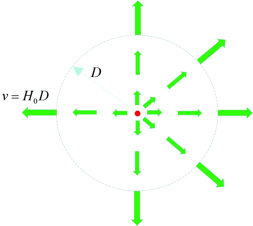
Fig. 1. In the FLRW model matter is distributed uniformly throughout the universe. The solution is maximally symmetric, no point is geometrically distinguished from any other. Every point in the universe sees the exact same motion of matter. In the figure, green arrows indicate the velocity field seen by a stationary observer at the center. Recession velocities increase (indicated by the longer arrows) with distance according to the Hubble law.

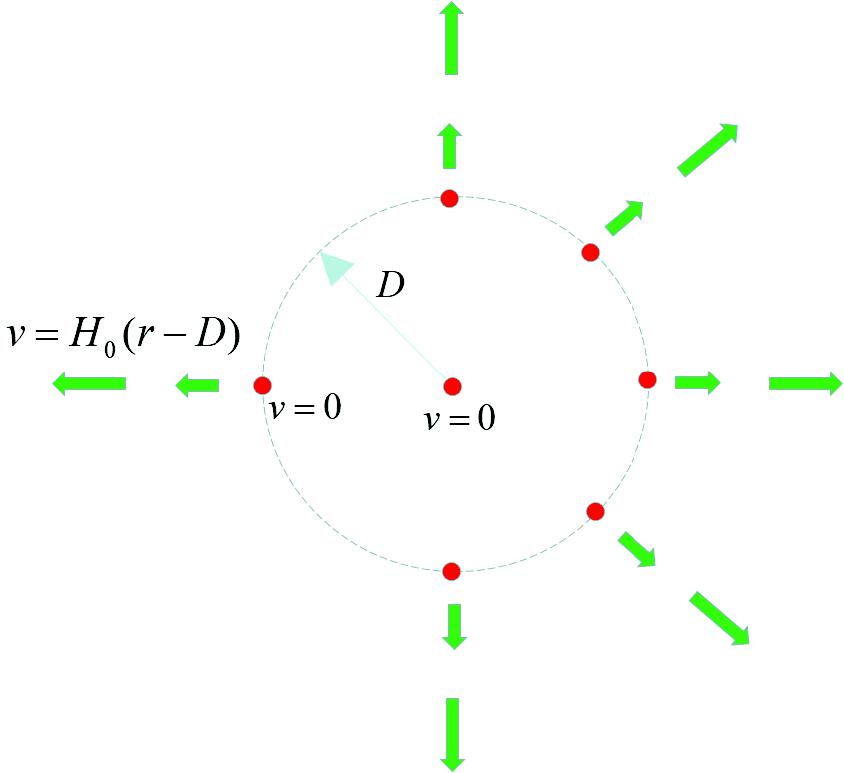
Fig. 2. In the cavity model matter is missing inside of R = D. Recession velocities increase (indicated by the longer arrows) with distance according to the Hubble Law outside R = D.

This motion of matter is contained in the calculation of the stress-energy of the universe. And the stress-energy in turn is the source of the gravitational field. Thus, the view emerges that matter (stress-energy) produces the gravitational field (and as such curvature) and that the curvature produces altered motions of matter in free fall (the inertial frames, geodesic paths). Such an interpretation is very satisfying and avoids giving occult powers to space—a notion contrary to the relativity principle of GR (fig. 3).

Fig. 3. Causal chain of Theory of General Relativity.

This Machian view is further enhanced by the fact that if it is space expansion that is the motive force, then even the sizes of objects should increase with the expansion of space. Such is not the case. Matter is not cemented to space by way of a dark epoxy.7 If one is committed to the expanding space paradigm, then it seems that one is also committed to a belief in absolute space and that all matter with zero peculiar velocities in the universe is at rest (motionless) with respect to the expanding absolute space. This is a rather peculiar interpretation that is at odds with the Machian relativistic point of view. In fact, as we show below, matter with peculiar velocities come to a state of rest with respect to the global flow. If it is space that is the reference frame then the natural state of matter in this interpretation would be the state of rest with respect to the absolute space. This is Aristotelian physics, and is at odds with the Machian interpretation of GR espoused in this paper.

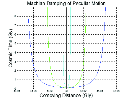
Fig. 4. Machian damping of peculiar motion in the open FLRW Model.

Fig. 4 is a plot of particles with peculiar velocities in the open FLRW cosmology that demonstrates the Machian dragging of particles by the global flow of matter. The trajectories were obtained by solving the geodesic equation of motion of particles. Each curve is a particle with differing peculiar motion at an initial time. The dark blue line has the greatest peculiar velocity, followed by the green lines and finally the light blue has the smallest peculiar velocity. The central black line is a particle with zero peculiar velocity. Note that as the expansion of the matter evolves, the peculiar motion is damped. Each trajectory asymptotically approaches a constant comoving coordinate, thereby joining the cosmic flow and at rest relative to the cosmic inertial frame (determined by the matter).

In the next section we introduce a simple cavity solution and show that the interior is a static (non-expanding) flat space. As a result, light travels at the special relativistic speed of light in cavities. There is no expanding matter in the cavity to drag the light. We then provide the details of solving the peculiar motions in the open FLRW homogeneous model and interpret the solution in terms of Mach’s principle. We will then compare the light travel time in the expanding homogeneous model with the travel time in the cavity and show that the expanding matter significantly increases the travel time to reach the earth. (The light has to swim against the inertial tide.)

Inhomogeneous Models

As was shown in Dennis (2018), spherically symmetric inhomogeneous models can be constructed in comoving coordinates. A good reference for this analysis is the seminal paper by Bondi (1947). To solve for an inhomogeneous cosmology with a cavity we will use Bondi’s (1947) equations.8

The metric interval for the general case of an inhomogeneous spherically symmetric space-time in comoving coordinates of freely falling particles is given by the form (using natural units):

(2)

This is a general isotropic and time dependent metric. Due to isotropy the metric is independent of the angular coordinates. Each particle is labeled by a fixed radial coordinate r (at an arbitrary time) and its constant angular location. These coordinates follow the particles and do not change, hence the term comoving. From this we see that the four-velocity of the matter at fixed (r,θ,φ)=(r₀,θ₀,φ₀) is:

From the normalization condition for time-like curves, we get:

This implies that if we choose the interval s (arc length parameterization) as the coordinate along the time like curves, then g₀₀=–1. Therefore, all clocks are radially free-falling at constant comoving coordinate r and thus register the cosmic time dt²=–ds², which would be the age of the particles. Note that R(t, r) is no longer a radial coordinate but a function of the comoving coordinate r and the proper time t. However, the area of a sphere at time t and radius r is still 4ΠR² (t, r).

Anticipating later discussion, we point out that this form of the metric in comoving coordinates excludes a broad class of physically realizable cosmologies. For many physical solutions the comoving coordinates break down and become invalid depending upon the initial energy conditions. We will point this out later.

The EFE with cosmological constant Λ=0 and a pressureless dust then reduce to the following set of independent equations (LTB model historically developed by Lemaître, Tolman, and Bondi):

(3) (4) (5)

In these equations M(r) is the gravitational mass within a radius r from the center of symmetry. It is not to be confused with the total invariant rest mass that appears in stress-energy tensor by way of the invariant density ρ. M(r) measures the rest mass energy plus (a negative) gravitational binding energy. For example, for closed solutions the total gravitational mass can be zero even though ρ (which is always non-negative) is not. E(r), which it is important to note, is a constant of integration. It is the energy and curvature at a given comoving radius r. E(r) is required to satisfy the inequality E(r)>–1/2. For E(r)<0 we have a closed universe with positive curvature which expands from an initial big bang to a maximum radius then collapses to a final big crunch. For E(r)=0 the universe is open and flat (zero curvature), while for E(r)>0 (and M non-zero) the universe is open and hyperbolic (negative curvature).9

Equations (3)–(5) only model the gravitational interaction; no other forces are modeled. The energy function E(r) is a constant of integration and is arbitrary. It would be the initial energy distribution of the universe as a function of the radial coordinate. This would be the initial energy distribution of the matter created by God.

Looking at equation (3) we see that it is remarkably Newtonian in form. If there is a region (cavity) where M(r) is zero for r<r₀, then the scale R is a linear function of time. This corresponds to a cavity wall moving at constant speed with scale:

It is important to note that in regions where there is no mass that the scale factor is entirely independent of any physical content. This is due to the fact that there is no matter that can be the carrier of the energy E(r). This shows that the choice of E in empty regions is merely mathematical. This too is consonant with Machian dragging. The comoving coordinate scale is only coupled to a physical effect when there is moving matter.

For simplicity we will examine the case for which the cavity wall is at rest. This case does not alter the conclusions. Allowing the cavity wall to expand at constant speed still yields that space is not expanding in the cavity, but rather the cavity wall is receding. In particular, we take E(r)=0 in the cavity (since M(r) is zero in the cavity).10 This choice corresponds to inertial test particles at rest in the cavity relative to the cavity wall. The test particles stay at rest since the interior is flat and static Minkowski space. It is devoid of gravity. So, E(r)=0 results in a continuous comoving coordinate system at the cavity wall. Clearly in this case of regions with no matter there is no expansion of space. This is consonant with the Machian view that matter is the source of the gravitational dynamics and the motion of matter, not space. We will elaborate on the above in Appendix C.

Observe also that equation shows that speeds greater that c are allowed in GR, since solving for the expansion rate gives:

Thus we see that GR does not preclude global velocities greater than the local speed of light. We should note also that the GR equations do not directly include other energy sources (except as modeled in the stress-energy tensor) since E(r) is an arbitrary constant not specified by quantities appearing in the EFE, thus it is possible that ultra energetic sources can also produce local superluminal expansions if they provide a sufficiently large value of E.

For the case of the cavity, we take the density ρ(t, r) at proper comoving cosmic time t₀ to be given by:

(6)

Here, ρ₀ is a constant.

Setting E(r)=0 (that is, we are taking the particles of matter to be free), we obtain from equation (3):

(7)

Choosing the time coordinate such that R=r at t=0, the solution of the equation (7) for R is then:

(8)

We can integrate eq. (5) to obtain:

(9)

Since ρ(0, r) is piecewise constant, we can move it outside the integrand, integrate over each constant region, and obtain:

(10)

Since

we obtain:

(11)

Note that based on equation (6), the cavity wall at R=r=r₀is constant in time. This we expect since there is no gravitational pull on the inner surface of the wall.

The metric for the expanding matter outside the cavity is thus:

(12)

Now consider the solution for r<r₀. There, M(r)=0, and equation (8) becomes:

(13)

So, the metric inside the expanding cavity reduces to:

(14)

Examining this solution, we see that inside the cavity the metric is static Minkowski space and space does not expand. This is one counterexample to the homogeneous fabric of space paradigm. We might consider how the expansion of space view was proposed. The claim of this author is that it is an artifact of comoving coordinates. Since comoving coordinates are constant for the cosmic dust, it gives the illusion that the dust is attached to the space, and thus since comoving coordinates are constant, it must be space that is expanding. The temptation to adopt this stems from the mistaken notion that special relativity trumps general relativity. It is the other way around, as the above analysis of the EFE shows. The reasoning behind the expanding space view is the claim that since nothing material can travel faster than light (meaning the value c from SR), then it must be the space that is expanding. The reason claimed for this is that space is not subject to the SR speed limit. However, proponents of expanding space provide no physical foundation for this ad hoc extraordinary claim.

Note that if E>0 then the cavity wall expands with constant speed

The physical speed at which the wall recedes is (we have reinserted the speed of light for clarity and ease of interpretation):

Since GR places no restriction on E (except that it is strictly greater than –¹⁄₂, as above), then for E>0 the value of v is unbounded. So, we see that recourse to the special relativistic speed limit that nothing can travel faster than the speed-of-light except for space is suspect.

In concluding this section, we note that once an incoming light ray reaches the cavity wall, it is no longer slowed by the receding mass, but travels through the cavity at the special relativistic speed c. We use this fact below in the comparison of travel time in a vacuum to the travel time in the globally homogeneous models. We also point out that the incoming photons traveling in the matter regions will exhibit redshifts while traveling through the matter regions (this follows from the standard redshift analysis), but there will be no more additional redshift as the photons traverse the empty region. We point out also that a more general cosmological solution consisting of numerous concentric regions of matter separated by voids will also exhibit a form of clumping of redshifts. These redshifts occur as the photons traverse the matter shells. Of course, more quantitative analysis is required to verify this conjecture.

This counterexample of an empty shell may not be entirely convincing to some. We now provide other counterexamples by analyzing in detail the method of coordinate construction in highly symmetric spacetimes11 and the issue of shell crossings in these cosmological solutions.

Shell Crossings in Cosmological Solutions

We return to an analysis of the manner in which the comoving coordinates are constructed and examine the restrictions that the metric functions must satisfy so that comoving coordinates remain valid. This analysis is based on the work of Hellaby and Lake (1985) that provides the conditions for no shell crossings in spherically symmetric cosmologies.

The analytical conditions for no shell crossings developed in Hellaby and Lake (1985) are relatively involved. The motivation for characterizing the conditions for no crossings is that shell crossings result in a violation of the conditions for the validity of comoving coordinates and that the coordinates are well behaved. We remind the reader that the basic conditions for coordinates are that they are real numbers and that the coordinates are 1–1 mappings in a neighborhood of a point in a manifold. If the 1–1 mapping is violated, then they cease to represent unique points in the manifold.

However, at this point, we are not interested so much in what mathematical conditions are needed for maintaining mathematically well-behaved coordinate systems. Such conditions, we will see, are too restrictive and eliminate many real physical solutions. In fact, the models for which comoving coordinates are meaningful are the spherically symmetric solutions (homogeneous and inhomogeneous) of the EFE. It is easier to construct shell crossing violations by straightforward physical considerations.

Such mathematical violations show that the comoving coordinates only allow a rather restrictive set of solutions (those with well-behaved initial conditions that exclude collisions of matter) and eliminate a vast collection of physically realizable solutions. The general (and less idealized) physical case is shells of matter that can cross (or separate). Simple examples would be: (1) an exterior imploding shell meeting an interior exploding shell, or (2) a free exterior shell escaping to infinity while an interior bound sphere collapses to a singularity.

Comoving coordinates are constructed via labels that are attached to the particles of the gravitational model. If a particle is moving, then its label does not change.12 So then, while comoving coordinates might be useful before the collision, once the crossing occurs the comoving coordinates cease to be useful. Let’s consider the situation analytically by examining equations , and above.

If we look at equation (2), we see that the function R(t, r) is the curvature function for a shell at comoving radius r at time t. The requirement for the coordinate system to be well behaved is that R is monotonically increasing as a function of the comoving coordinate r. If this is not the case then we have the case of shell crossings since we would have a decrease in the surface area of the shell when r increased, indicating that a shell of a given r has collapsed to a sphere with less surface area. As explained by Hellaby and Lake the condition for incipient shell collapse is Rʹ=0. This indicates a surface where an increase in comoving r coordinate does not increase surface area. If we have a solution for which Rʹ=0 it is not a violation of the physics. Rʹ=0 is allowed by the field equations and the chosen initial conditions.

The coordinate singularity at a shell crossing can be seen from equation (4). If Rʹ=0 then the metric component g_rr=0 indicating a degenerate metric. The singularity is also evident from the 4D volume element:

Indicating that the volume of the 4D coordinate extensions is 0.

The above analysis alone should be sufficient to overturn the expansion of space paradigm. Reflection on the fact that the coordinates are attached to the particles, shows that shell crossings are shells of matter crossing each other. It is not a case of space crossing itself resulting in the development of topological defects in spacetime. It is merely an indication of conditions that invalidate the coordinate construction. Comoving coordinates become invalid when the shells of matter cross or separate.

That we can construct such violations in a physically meaningful way follows easily from the energy term in equation (3) above. As mentioned, E(r) is an arbitrary function of r.13 If E transitions at some value of the comoving r from a non-negative value to a negative value (at a larger value of r) we have the physically realizable solution. It represents an outgoing shell of matter surrounded by an imploding (bound) shell of matter. Clearly these shells will collide. The collision is a collision of matter not a folding of space back on itself.14 The collision is a case where comoving coordinates are invalid. This shows that the idea of expanding space from a naïve interpretation of an abstract coordinate system in a highly idealized cosmological model is an illusion and mistaken.

Expanding on the above, we describe two configurations of matter and energy distribution that result in breakdowns of the comoving coordinates. These configurations, which follow easily from a consideration of the energy domains and dynamics of gravitating systems, are: (1) a gravitationally bound sphere of homogeneous matter surrounded by a gravitationally free homogeneous distribution of matter, and (2) a gravitationally free sphere of homogeneous matter surrounded by a gravitationally bound homogeneous distribution of matter. In both of these scenarios the two regions are initially contiguous so that the comoving coordinate is continuous and the radial scale factor R is also continuous. We take the boundary of the two energy regions to be at comoving r=r₀. The energy equation (3) above can be analyzed exactly as in the Newtonian case.15 Solving for the radial speed we get:

(15)

This yields that for E(r)<0 there is a maximum radius for each comoving shell at radius r:

The shell reaches it maximum expansion then collapses, such that . For E(r)>0 and positive initial shell speed, there is no maximum radius and all shells escape to infinity.

In case (1), the inner sphere collapses, while the external matter expands. This results in shell separation or the creation of a gap (a void) between the two energy regions, yet there is no comoving coordinate that applies within the gap. In fact, the coordinate r₀ is attached to both the surface of the collapsing shell, and also to the cavity wall of the expanding exterior matter. This scenario is depicted in fig. 5.

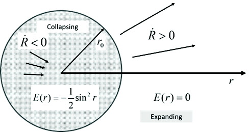
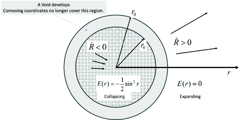
Fig. 5. Homogeneous matter distribution with two different energy regions. A. Initial condition. Bound interior and free exterior. B. Configuration as the system evolves. The interior collapses and exterior expands creating an empty void with no coordinates assigned.

In case (2), the inner sphere expands to infinity, while the external matter collapses to a singularity. This solution of the EFE uses the positive branch of equation for the inner sphere and the negative branch for the external matter. This results in shell crossings that develop at r=r₀, and a merging of the matter of the two energy regions. In the overlap there are two values of r attached to each point within in the overlap. The mass distribution and energy distribution functions are no longer valid there and consequently the radial factor _R(t,r) is no longer a valid representation of the geometry in the overlap. There is no comoving coordinate that is valid within the merging region. In fact, the coordinate r⁰ is attached to both the surface of the expanding sphere, and to the cavity wall of the collapsing exterior matter. This scenario is depicted in fig. 6.

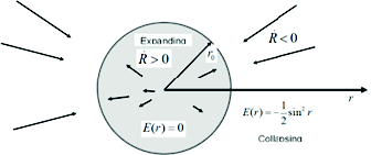
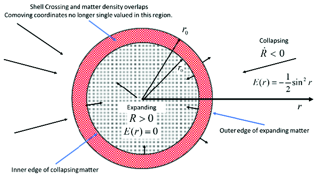
Fig. 6. Homogeneous matter distribution with two different energy regions. A. Initial condition. Free interior and bound exterior. B. Configuration as the system evolves. The interior expands and exterior collapses creating a merger of the matter with no unique coordinates assigned.

Homogeneous FLRW Cosmologies

We return now to the analysis of the large light travel times in a homogeneous expanding universe. The homogeneous model can be obtained from the inhomogeneous model by restricting the density to a function of time only. In this case the radial scale simplifies to:

With this simplification, the global homogeneous FLRW solution in comoving coordinates becomes:

(16)

The function f_k depends on the curvature index k, which in turn is determined by the energy of the particles.

Recall that K=1 is the bound solution with positive curvature, K=0 is the open and flat solution, and K=–1 is the open solution with negative curvature.

The free-falling particles are governed by the geodesic equations. For the homogeneous models these equations are:

For simplicity, in the subsequent analysis, we will consider only radial motion. Thus, the angular velocities are 0, and we have the following two equations for the trajectory in (t,r):

(17)

Inertial Dragging in Homogeneous FLRW cosmologies

In this section we illustrate by quantitative analysis that particles with peculiar velocities undergo acceleration relative to the comoving Hubble flow.16 This is expected from Mach’s principle since the global Hubble flow of free-falling matter is the cosmic inertial frame. It is important to note that the particles with peculiar velocities are also in free fall, yet their motion is altered to approach the Hubble flow’s local rest frame. We explain this as due to the cosmic time-dependent gravitational field which manifests itself as a time-dependent constant curvature.

The equation for r yields the constant of the motion:

(18)

For particles with constant r (that is, the Hubble flow, or zero peculiar velocity) a=0. For a particle with a non-zero peculiar velocity given by:

we get the first indication of Machian inertial dragging since:

(19)

This shows that the peculiar velocity of a particle changes inversely to the scale of the universe. In particular for the open expanding solutions for which a approaches infinity, the peculiar velocity approaches zero. Thus, peculiar velocities are damped and the particle motion will asymptotically converge to the Hubble flow.

To aid in the solution of the geodesic equations we use the metric normalization of the four-velocity to produce the quadrature (for radial motion):

Substituting into gives another expression for the peculiar velocity:

Particle Dynamics in the Flat FLRW Solution

For simplicity in the following analysis, we restrict attention to the flat solution with zero curvature, K=0. This model is also more in line with current assessment of the large scale geometry of the universe. For the flat solution, we have (see for example, Misner, Thorne, and Wheeler 1973):

(20)

We choose r to be a physical distance, so that the scale factor a is dimensionless.

Solution of the Friedman equation for spatially homogenous matter density, gives:

(21)

The constants of integration have been chosen so that the singularity occurs at time 0 and such that the scale factor is unity at a present putative time of 1/k. This choice means that the constant comoving coordinates are the proper distances of objects at the current time (epoch). Note that ρ₀ is the cosmic density at the current epoch, when a(τ)=1.

To see the effect of Machian dragging in detail, we expand the derivative in equation :

Substituting equation (18) gives:

This shows that test particles with peculiar velocities (a≠0) experience kinematic acceleration relative to the motion of the Hubble flow. However, such particles experience no dynamic acceleration since they, too, are in free fall and inertial. Accelerometers would register zero acceleration.

As time increases, the second term approaches zero, since the derivative of the scale factor a(t) is:

Therefore, the motion of the object in comoving coordinates approaches

These quantitative features were illustrated in fig. 4.

Light Travel Time in Homogeneous FLRW Cosmologies and Cavity Models

In this section we derive the time of flight of photons in the open FLRW model and compare the time to the time to travel the same distance in a cavity (vacuum). We choose the open solution since it more closely matches current observations of a nearly flat universe and the results are easier to interpret than using the standard model.

Photon trajectories are determined by ds²=0, which is:

(22)

The plus sign is for outgoing light and the negative sign is for incoming light.

Consider an incoming photon emitted at time τ₀ from a distant source at a comoving distance r₀ and arriving at r=0 at time τ. Its trajectory is obtained by integrating equation 22:

Yielding:

After some algebra, this can be solved for the travel time, τ–τ₀

(23)

Note that r₀ is the current distance at epoch; it is not the physical distance of the source at time of emission. The physical distance at time of emission is:

Using this to eliminate r₀ we obtain:

Note that the leading term is independent of time of emission. It is the time a photon would take to traverse a void of size D_0. Therefore the ratio, R, of the FLRW time of flight to the cavity (vacuum) time of flight is:

(24)

Finally, introducing the notation

(25)

The two expressions in equation will allow us to express ζ in terms time of emission and proper distance at emission or comoving distance.

Using equation (25) then yields the simple formula for the ratio of the homogeneous universe travel time to the vacuum travel time:

(26)

This shows that the travel time increases quadratically as ζ. Since ζ increases with proper (or comoving) distance and with decreasing times of emission, we see that the travel time from distant objects at early times is strongly slowed by the homogeneous expanding matter of the Hubble flow, thus the reciprocal of equation (26) gives a formula for the reduced travel time in cavities.

Another useful quantity is the effective speed of light. We note from equation (24) that the reciprocal of R is the total proper distance (at emission) divided by the time of flight, which is the effective speed of light.

In the next section we analyze the results of this analysis.

Before we do so, we present in fig. 7 an illustration of photon trajectories in the open FLRW cosmology using physical distance as the radial coordinate, rather than the comoving distance. In Appendix B we derive the expression for the metric in terms of physical distance. This figure’s illustration of superluminal physical speeds may be the most important in this paper. The figure plots the proper (physical) distance of the photon from an observer as a function of cosmic time. Recall that the proper distance D at time t is related to the comoving distance r via:

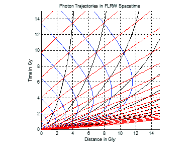
Fig. 7. Trajectories of incoming (blue) and outgoing (red) light rays in open FLRW model. Black lines are trajectories of the Hubble flow.

Blue lines are incoming photons and red lines are outgoing photons. Note that early in the expansion, incoming photons are actually receding from the observer (proper distance is increasing). This is due to the inertial dragging of the light by the time-dependent gravitational field of the Hubble flow. The photons reach an apogee and then finally approach and reach the observer at the origin. For example, the light trajectory that arrives at the earth at time 9 Gy receded to an apogee of 4 Gly at approximately 2.5 Gy. This delay in approaching the observer is due to the Machian effect. There would be no delay in the absence of the Hubble flow. Note that the diagram shows that the trajectories of the massive particles (indicated by the black lines) always lie inside the null cone. This is in keeping with our remark that even though the massive particles are globally traveling with a speed greater than c they do not travel faster than the local light. Note also that the null cones (and the matter trajectories) are tilted more severely toward increasing distance as time approaches zero—another indication of the global speed of the matter traveling faster than the special relativistic value of c. One final comment: note that near the event at distance 2 Gly at time 12 Gy, the light speed is c (as indicated by the 45° slopes of the incoming and outgoing light trajectories). In the near neighborhood, and at late times (when the matter speed is becoming smaller) the amount of inertial dragging of the light has decreased significantly.

Results

In the following we present the results via several plots that give: (1) time of flight as a function of both proper distance and comoving distance; (2) ratio of homogeneous time of flight to the cavity time of flight; (3) effective speed of light in the open FLRW cosmologies.

We plot the ratio of the time of flight of incoming light given in equation for representative values of proper distance and time of emission. Rather than using the currently estimated density at epoch of ρ₀=9.9×10^–27kg/m³
obtained from the standard cosmology, we will select the density for the open FLRW such that the age computed fits the current old universe value of 13.8 Gyr. This gives ρ₀=4.2×10^–27kg/m³. For comparison we will plot the results for light travel within a young age cosmology and the old age cosmology. Also, for each case, we plotted several measures of the light travel time as a function of distance (both comoving and proper distance) and emission time. When interpreting the graphs, it is important to remember that the comoving distance is the theoretical distance according to the model where the object would be today. In the graphs, the proper distance is the distance of the object at time of emission. The latter provides an easier calculation of the effective speed of light as the proper distance at emission divided by the travel time. The measures we selected are: (1) total light travel time; (2) ratio of travel time in matter to that through a cavity of the same distance; and (3) the effective global speed of light (compared with c, the speed through a cavity).

For each of these measures we note the following related results. The total light travel time traveling through matter is always greater than the cavity time. Thus, the ratio mentioned above is always greater than 1; and, finally, the effective global speed of light in matter is always less than c.

Results for a distance of up to 1Mly are graphed in fig. 8 using emission times within a YAC time scale. The reduction of time of flight is shown for four emission times. The travel time in a void is reduced by a factor on the order of 10⁴. This is significant. However, it should be noted that the time to travel 1Mly in the vacuum is still 1 million years.17 The figure shows that the time for light emitted 1,000 years after creation to traverse the 1Mly distance in a homogeneous matter distribution would be approximately 35 billion years. The main point is that though cavities in themselves do not bridge the entire LTTP they do significantly reduce travel time compared to that predicted by the globally homogeneous models.18 Thus, exploration of cosmological models with many voids should be a fruitful line of research.

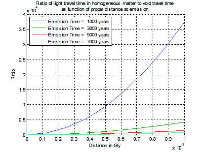
Fig. 8. Ration of light travel time in open FLRW cosmology to a vacuum cavity.

In fig. 9, the light travel time in the homogeneous open FLRW cosmology is plotted as a function of proper distance (A) and comoving distance (B). In fig. 9(A), travel time for a proper distance at emission clearly shows that the expansion of matter results in travel times much greater than the equivalent time through a void (indicated by the lowermost black line). This result is also illustrated in fig. 10 which plots the ratio of light travel time in the homogeneous matter cosmology to that in a void. The ratio is always greater than 1.

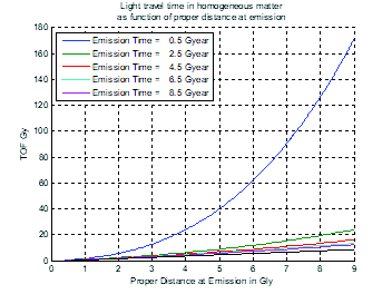
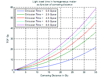
Fig. 9. Light travel time in open FLRW cosmology as function of emission time and proper distance (A) and comoving distance (B).

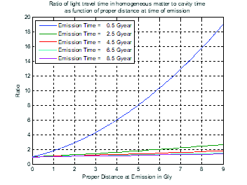
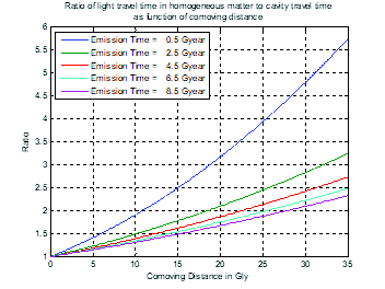
Fig. 10. Ratio of speed of light in homogeneous open FLRW model to speed in vacuum.

In fig. 11, the effective speed of light, defined as total proper distance traveled from the source to the origin divided by the total time, is plotted for several emission times and comoving distances. The figure shows that the effective speed of light is much less than the vacuum local speed of light of special relativity (speeds are normalized to c=1). The graph shows that the effective global speed decreases as proper distance increases and also for earlier emission times. This is understandable as the speed of the Hubble flow increases for earlier times of emission (the expansion of the matter is more rapid in the early stages of the expansion before slowing due to gravitational pull).

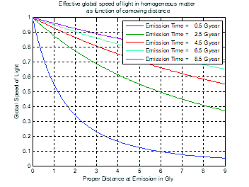
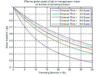
Fig. 11. Effective global speed of light as function of proper distance (A) and comoving distance (B) and time of emission.

Conclusions

We have shown that the cosmologies with homogeneous expanding matter lead to light travel times that are significantly greater than the travel time traversing cavities. A main point is that space in cavities does not expand and that empty space cannot impede light transit to the earth. Thus, inhomogeneous cosmologies with large voids will have significantly less light travel times than those predicted by the homogeneous cosmological models, such as the standard model. We also examined how Mach’s principle provides a satisfying explanation of the physical effects in a way consistent with the principles of GR. We quantitatively provided counterexamples to the expansion of space paradigm via the inhomogeneous cavity cosmology and the Hellaby and Lake analysis of the general breakdown of comoving coordinates. Another important point is that “superluminal” global speeds are adequately explained within GR without recourse to the space expansion argument. We have shown that an appeal to the SR speed limit for global speeds in GR is misguided. GR is the covering theory of SR and SR is to be interpreted in light of GR, not the reverse. We demonstrated that nothing in GR precludes global velocities greater than the local speed of light.

In light of these considerations, we believe the expanding fabric of spacetime concept (given that it means empty space can expand) should be abandoned by YAC cosmologists; it is inimical to young age creationism as it results in longer light travel times even in voids. This means that the use of voids should decrease the light travel times predicted by the inhomogeneous model I presented in Dennis (2018). This is because my 2018 model still had regions of expanding matter in the neighborhood of the earth (though of lower mass density than the remote universe). I hope to explore these refinements and an analysis of reduced light travel time in my inhomogeneous model in a future paper.

Acknowledgments

The author thanks John Byl, Danny Faulkner, Robert Walsh, and an anonymous reviewer for their comments and discussions that have helped improve this paper.

References

Barbour, Julian and Herbert Pfister. 1995. Mach’s Principle: From Newton’s Bucket to Quantum Gravity. Basel, Switzerland: Birkhäuser.

Bondi, H. 1947. “Spherically Symmetrical Models in General Relativity.” Monthly Notices of the Royal Astronomical Society 107, nos.5–6 (December): 410–425.

Davis, Tamara M. and Charley Lineweaver. 2004. “Expanding Confusion: Common Misconceptions of Cosmological Horizons and the Superluminal Expansion of the Universe.” Publications of the Astronomical Society of Australia 21, no.1 (5 March): 97–109.

Dennis, Phillip W. 2018. “Consistent Young Earth Relativistic Cosmology.” In Proceedings of the Eighth International Conference on Creationism, edited by J.H. Whitmore, 14–35. Pittsburgh, Pennsylvania: Creation Science Fellowship.

Frolov, Valeri P., and Igor D. Novikov. 1998. Black Hole Physics: Basic Concepts and New Developments. Dordrecht, Netherlands: Kluwer Academic Publishers.

Gullstrand, Allvar. 1922. “Allgemeine Lösung des Statischen Einkörperproblems in der Einsteinschen Gravitationstheorie.” Arkiv för Matematik, Astronomi och Fysik 16, no.8: 1–15.

Hellaby, Charles, and Kayll Lake. 1985. “Shell Crossings and the Tolman Model.” The Astrophysical Journal 290 (March 15): 381–387.

Johnson, Bryan M. 2018. “Towards a Young Universe Cosmology.” In Proceedings of the Eighth International Conference on Creationism, edited by John H. Whitmore, 46–51. Pittsburgh, Pennsylvania: Creation Science Fellowship.

Krasiński, Andrzej. 1997. Inhomogeneous Cosmological Models. Cambridge, United Kingdom: Cambridge University Press.

Mach, Ernst. 1989. The Science of Mechanics. 6th edition. Chicago, Illinois: Open Court Publishing.

Misner, Charles W., Kip S. Thorne, and John Archibald Wheeler. 1973. Gravitation. San Francisco, California: W.H. Freeman.

Mukhanov, Viatcheslav. 2005. Physical Foundations of Cosmology. Cambridge, United Kingdom: Cambridge University Press.

Nielsen, N.K., 2022. “On the Origin of the Gullstrand–Painlevé Coordinates.” The European Physical Journal H 47, no. 1 (9 May), article 6.

Painlevé, Paul., 1921. “La Mécanique Classique et la Theórie de Relativité.” Comptes Rendus Academie des Sciences 173: 677–680.

Peacock, John A. 1999. Cosmological Physics. Cambridge, United Kingdom: Cambridge University Press.

Peebles, P.J.E., 1993. Principles of Physical Cosmology. Princeton, New Jersey: Princeton University Press.

Sachs, M. and A.R. Roy. 2003. Mach’s Principle and the Origin of Inertia. Montréal, Québec: Apeiron.

Appendix A.

Derivation of Local and Global Speed-of-Light

There are many representations of the FLRW metric in the literature (see, for example, Krasiński 1997). For our derivation we write the metric of the FLRW model with scale factor a(t) as a function of cosmic time t as:

The distance D of an object at constant comoving coordinate at cosmic time t is obtained by integrating the proper spatial interval within a t=constant surface along a radial direction.

Taking the time derivative, the global speed of the Hubble flow at that point is:

It is well known that this speed can be larger than the local speed of light value c of special relativity.

For photons, r is not constant. In fact for photons we have:

So

Thus, the global speed of incoming and outging light is (⁺ for outgoing; – for incoming):

(27)

Thus, subtracting the speed of the Hubble flow, that all matter exhibits, yields the local speed of light:

c_local = v_light – H₀D = ± c

Appendix B.

Derivation of the Metric in Physical Coordinates

We derive the metric for the open FLRW solution in terms of the physical distance instead of the comoving coordinates.

From equation (4) the physical distance ρ from the origin is given by:

For the open FLRW case (with E(r)=0) we have:

Thus, the coordinate transform to physical distance is:

Taking the differential yields

Solving for dr in terms of dt and d ρ and substituting in equation (20) yields:

(28)

Here,

is the Hubble constant. In this case we see that the factor

(29)

represents a time dependent gravitational field. This factor shows that there is a Hubble horizon at distance (inserting the speed of light) :

This is the maximum distance at which the physical coordinates constitute a valid coordinate system.

Solving equation (28) for the photon trajectories (ds=0), yields the global physical speed of light (with respect to the clock at the origin):

(30)

This is the global physical speed of light as also derived in Appendix A. The first term is the dragging of the light by the expanding matter and the second term is the local (peculiar) speed of light. Note that objects beyond the Hubble horizon cannot be seen since, from equation (30), all light has positive recession speeds, and never reaches the origin.

Equation (28) is the metric that corresponds to fig. 7 of the main text. An interesting aspect of this metric is that the 3D metric of the spatial geometry,

at each instant is static and Euclidean, thus reinforcing the view that space is not expanding.

We can use the dependence of H(t) on the matter density to transform equation (28) to an interesting form.

From the EFE we have19

This gives:

In which M(t) is the amount of mass inside a sphere of radius ρ at time t.

Substituting into equation (28) yields:

(31)

This is the Gullstrand-Painlevé coordinate form of the Schwarzschild solution with a time dependent mass.20 The function M(t, p) is the mass inside of fixed radius at time t. The mass depends on time since as the matter expands in the static spatial geometry the amount of mass inside a sphere decreases.

We see that for an observer at fixed distance the geometry looks like a Schwarzschild solution with time dependent mass. A further interesting aspect is that an observer at fixed distance is not a geodesic, and not an inertial observer. Thus, to maintain the fixed distance, the observer must apply an acceleration. This acceleration is needed to counteract the Machian drag produced by the inertial Hubble flow. Thus, this form of the solution further supports the Machian viewpoint of this paper.

Appendix C.

The Milne Model, Other Cavity Coordinates Derived From E>0 in the Interior, and Other Comoving Coordinates

In the main text I chose a particular choice of E(r)=0 since it was mathematically convenient and manifested the geometry of Minkowski spacetime in the interior. This choice was in part motivated by the physical consideration that there are no carriers of energy in the cavity. Also, such a choice provided a continuous coordinate system that joined smoothly to the static cavity wall. This is illustrated in fig. 12. As the figure shows, the timelike worldlines of the interior test particles correspond to particles at rest inside the cavity. Inside the cavity, r measures the distance in the cavity from the origin. That distance is time independent. Clearly, the cavity is not expanding. Below we will choose the Milne coordinates that seem to imply the interior is non-static and that space is expanding. At this point, we merely remark that the interior space cannot be both expanding and not expanding at the same time depending on the choice of coordinates. Coordinates per se are not imbued with metaphysical powers to warp space.

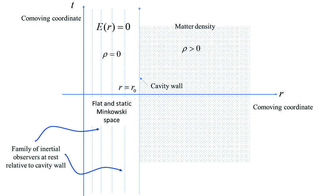
Fig. 12. Illustration of the continuous coordinates of the cavity model consisting of exterior free matter escaping to infinity. Figure shows intertial “test particle” trajectories in the interior. Such “particles” are not physical they only provide a coordinate chart for the interior Minkowski spacetime.

However, for completeness, in this appendix we discuss the cases of other choices of the energy constant E(r) in the cavity interior. We show that such choices do not alter the conclusions of the main text. Some choices result in discontinuous coordinates that serve to strengthen the Machian viewpoint.

As we noted, the geometry of the cavity interior is intrinsically Minkowski spacetime, which is flat and static. Geometrically it is symmetric under the 10 parameter Poincare group. Choosing different functional forms for E only results in change of coordinates of Minkowski spacetime. We will show that such coordinates cannot alter the symmetries of the interior under the Poincare group. This fact should be obvious since the Riemann tensor in the interior is identically zero. By the linear transformation law for tensors, under a change of coordinates, a zero tensor remains zero.

The different functional forms correspond to massless test particles which provide an infinite variety of comoving coordinates. Many of these are useless while others yield an illusion of a non-static interior. One such case is the Milne model which we now discuss.

The Milne Model

First, for the cavity interior we consider the choice:

(32)

An immediate observation is that this form is discontinuous at the static cavity wall which is the interface to the exterior where I took the matter to be expanding according to the gravitational energy integral with E=0, viz:

We note that there is no requirement that E be continuous, however such discontinuities result in the shell crossings explained in the main text. Such shell crossings in comoving coordinates in the case of fictitious test particles in the interior have no physical meaning. They merely point to the breakdown of the coordinates (in this case the Milne coordinates) at the boundary. We will show this to be the case.

For the interior, with M(r)=0 and equation (32), we obtain:

This yields the solution:

(We have dropped a constant of integration that merely specifies the time at which R=0). The positive value yields an expanding Milne model, the negative sign an imploding Milne model. We consider the positive case. Substituting into equation (4) gives the local coordinate form of the interior metric:

At this point we relabel the coordinates so that we do not inadvertently conflate them with the Lorentz frame coordinates in Minkowski space. The geometric significance has changed from the t and r used for the E=0 case. This is evident since the coefficient of the radial term shows that r is no longer a physical distance. For the new coordinates we make the replacements t→τ and r→ρ. This gives:

This appears to make the interior non-static. But the geometry in the interior is still flat static Minkowski space.

We transform to a new radial coordinate:

This gives:

This solution is shown in fig. 13. We first note that the Milne particles are a spherical spray of fictional particles emanating from the origin at time t=0 and expanding in time with constant speed. These are geodesics of Minkowski space. Each fictional particle has a speed that mimics a Hubble expansion, In the figure we show that the coordinates constructed via the Milne particles only cover that portion of Minkowski space in the interior of the future light cone. The figure also illustrates the shell crossing which occurs at the event labeled C (the explosion). This explosion is a collision of a fictitious particle with the cavity wall, not a physical shell crossing as in the main text. Consequently, it is a mere mathematical singularity. At that collision point the external and internal coordinates represent two different coordinate charts. We emphasize again that the shell crossings discussed in the main text were crossings of actual matter, represented by turning points in the mathematical scale factor of the comoving coordinates that track the matter.

This model of expanding observers in the Milne universe is nothing more than a different way to construct a coordinate system that covers a subset of Minkowski space within the cavity (namely the interior of the future light cone). These coordinates mimic a non-static and expanding empty universe which never slows down as there is no gravity to slow it down. It is nothing more than a spray of geodesics in Minkowski space (all traveling in constant speed straight lines with speed increasing according to a Hubble law). The figure shows the limited coverage of Minkowski space, viz. the region within the cavity and outside of the future null cone (the space like region relative to the origin labeled S in fig. 13) is not covered by the Milne coordinates. These moving fictional particles in Minkowski space (with their associated coordinates) can no more create a time dependent spacetime than various alternate coordinate systems for the surface of the earth can make the earth flat.

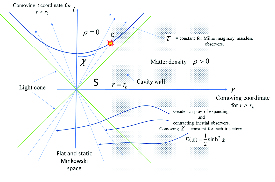
Fig. 13. Illustration of use of Milne coordinates in the interior cavity. The test particles (which have no physical significance to the cavity solution) only provide a different set of coordinates for Minkowski space. The interior geometry is still flat and static. The time dependence is only due to the motion of the test particles. The interior Minkowski space is not expanding.

We can transform back to the E=0 Lorentz frame from Milne comoving coordinates via:21

From this we determine that the speed of the test particles at comoving coordinate χ is:

We now prove that any choice of E(r) in an empty cavity yields the geometry of Minkowski as in special relativity (the theory with zero gravity).

General Proofs

As mentioned, different choices of E in regions for which M(r) is zero, always produce solutions that are the Minkowski geometry. The proof in general is tedious if calculated by hand but it is a straightforward computation of the Riemann tensor. Use of a symbolic computation program makes the task a breeze.

From equations (3) and (4), with M(r)=0, gives the solution:

(33)

E is an arbitrary function of r. The general expression for R is then:

The constants of integration have been chosen so that R=R₀ at t=t₀ .

From equation (33) we can compute the Riemann tensor. The answer is that Riemann=0 is independent of the function E(r). Thus, the calculation of Riemann proves that the interior is flat and static Minkowksi space showing that E(r) only specifies a coordinate system when M=0. One cannot make a static space into a non-static one and claim space expansion by a choice of comoving coordinates attached to imaginary particles in expanding motions through empty space.

A final general proof follows from Birkhoff’s theorem for the uniqueness of the geometry of a static spherically symmetric empty spacetime. That solution in Schwarzschild coordinates is the familiar expression:

For a region with no central mass M=0 yielding:

This is Minkowski spacetime, which is the unique geometry of a spherical region devoid of matter.

The Expanding Cavity Solution

The reader may wonder how an expanding cavity affects the above analysis. The answer is that the above arguments are all local, they depend only on the local density of matter at a location. The result is that the expanding cavity wall does not alter the analysis. In the cavity the local density of matter inside a sphere of radius r is zero. It does not matter if the exterior cavity wall is expanding with E>0. The geometry in the cavity is Minkowski spacetime. The Riemann tensor is zero.

Other Comoving Coordinates: Novikov Coordinates for the Schwarzschild Solution

Another example of comoving coordinates that seems to impart time dependence to static solutions is the case of Novikov coordinates. The detailed mathematics of Novikov coordinates can be found in Misner, Thorne, and Wheeler (1971, 826–827) and Frolov and Novikov (1998, 646–647).

Novikov coordinates correspond to freely falling test particles in the Schwarzschild geometry. In fact, the Schwarzschild solution in Novikov coordinates can be obtained from the LTB equations (equations [3]–[5]) in the main text, using the following expressions:

These choices yield the time dependent metric tensor in terms of the parametric equations:

Eliminating the cycloidal time parameter η then gives the implicit expression for R(t, r):

It is well known that Birkhoff’s theorem yields the result that the Schwarzschild geometry is the unique static geometry for a spherically symmetry gravitating source of mass M. The important point in this example is that the freely falling representation of Novikov coordinates results in a time dependent metric though the geometry itself is static. It is not surprising that infalling test particles see a time dependent metric. The test particles are moving through a spatially varying curvature and thus see a temporally varying curvature as they fall.22 Such time dependence is not surprising and unremarkable in itself. The point is that time dependence in a coordinate representation of the metric tensor does not imply a non-static metric.23

Conclusion and Summary

The above analysis shows that the spacetime in the interior of an empty spherical cavity is static and does not expand. This follows from: (1) the computation of the Riemann tensor in the interior for arbitrary “energy” functions, E(r). For the empty space inside the cavity the choice of E(r) does not alter the geometry; (2) Birkhoff’s theorem for the uniqueness of the geometry of a spherically symmetric spacetime. The unique Minkowskian geometry is obtained by setting M=0 in the Schwarzschild metric formula.

In conclusion, this analysis shows that the expansion phenomenon only occurs in regions where there is matter. In those regions, the expansion is an expansion of matter, not space, and the gravitational field of the expanding matter exerts a dragging effect on matter as discussed in the main text.