

Research conducted by Answers in Genesis staff scientists or sponsored by Answers in Genesis is funded solely by supporters’ donations.
Abstract
In recent years, the young-earth creation (YEC) model for human origins has made great strides showing that human history is stamped all over our DNA, and in a manner consistent with the YEC timescale. One of the most fruitful arenas has been the history of the indigenous peoples of the Americas. Previous Y chromosome work has confirmed the known post-Contact history and discovered migration events in the pre-Columbian era. In this study, I replicate these Y chromosome findings in the field of human mitochondrial DNA (mtDNA). I also extend the history deep into the past and solve some of the lingering questions raised by the initial Y chromosome findings. Finally, I show new evidence for a mtDNA root, and for the validity of mtDNA as a molecular clock.
Keywords: Mitochondrial DNA, pre-Columbian, Native American, Maya, Olmec, young-earth, evolution, molecular clock, origins, genetics, DNA, Y chromosome
Introduction
In recent years, the young-earth creation (YEC) model for human origins has made great strides testing some of its most obvious predictions: That human history should be stamped all over our DNA, and in a manner consistent with only around 4,500 years of history since Noah. In fact, this pursuit has been so successful that it has led to the genetic discovery of Noah himself. Genesis 10 describes the genealogy of the first several male generations after Noah. Analysis of the base of the male-inherited Y chromosome DNA tree shows a precise replica (Jeanson 2022).
Like all good scientific discoveries, these findings have led to even more testable predictions. One of the most fruitful subfields in this respect has been the history of the Americas.
The post-Columbian history of the Americas has a well-documented—though contentious—population trajectory. Middle-of-the-road estimates put the population size in the Americas in AD 1491 around 50–60 million (Denevan 1992). Then, in the centuries following, the indigenous population declined by 80% to 90% (Mann 2005). Among some indigenous American populations, numbers have begun to recover (McEvedy and Jones 1978). The YEC model has successfully captured all aspects of this history (Jeanson 2020; Jeanson 2022).
These successes have permitted the YEC model to penetrate one of the last great mysteries of human history: The pre-Columbian history of the Americas.
Mainstream science posits a single migration—or cluster of migrations—from Asia into the Americas about 15,000 years ago, followed by continuous habitation of the hemisphere up to the present (Potter et al. 2018). In YEC terms, “15,000 radiocarbon years ago” likely corresponds to the very early post-Babel time period, not more than a few thousand years ago. Thus, the YEC model would agree that people have been continuously in the Americas since the earliest times.
But the YEC model would not agree on a single migration. In the AD 300s to 600s, around the same time that the Huns were invading Europe and the Xianbei were assuming control of northern China after the fall of the Han Dynasty, another group of Central Asians crossed into the Americas (Jeanson 2020; Jeanson 2022). Y chromosome haplogroup Q documents this event. Y chromosome haplogroup Q also remains the dominant indigenous American Y chromosome haplogroup to this day (Jeanson 2022).
Conversely, in the AD 900s, while assorted Turkic peoples and Magyars were in the process of migrating into Europe and eventually dominating the Y chromosome haplogroups of modern Europeans, another group of Central Asians entered the Americas and gave rise to the Algic language family of indigenous nations (Jeanson 2022; Jeanson 2025). Y chromosome haplogroup C documents this event. Among Canadian First Nations, the majority of whom belong to the Algic language family, Y chromosome haplogroup C remains the dominant indigenous American Y chromosome haplogroup (Jeanson 2025).1
Curiously, at least one indigenous American document echoes the latter event: The Red Record or Wallam Olum (McCutchen 1993) of the Delaware, whose language belongs to the Algic language family. Careful reconstruction of the history in the Red Record shows a clear-cut match to the history in Y chromosome haplogroup C, as well as to oral histories (now written down) of other indigenous American nations (Jeanson 2025).
These advances have allowed, within a YEC model, the reconstruction of a detailed, play-by-play history for the last several centuries of the pre-Contact American period (Jeanson 2025).
But there remains a glaring hole in this model: The history of the Americas before the arrival of haplogroup Q. Archaeology describes a rich period of Central American history in the BC era. For example, in the second millennium BC in Central America, the Olmec civilization rose and flourished (Coe and Koontz 2013; Coe and Houston 2022). One of the most enduring legacies of the Olmec are their giant sculpted heads (Diehl 2005). The Preclassic Maya rose in the first millennium BC (Coe and Houston 2022). Recent LiDAR work has uncovered some of the magnificent accomplishments of the Preclassic era, including a network of cities connected via paved causeways (Hansen et al. 2023). One of the biggest cities of pre-Columbian Mesoamerica, Teotihuacan, traces its origins to the late first millennium BC (Cowgill 2015; Gorenflo, Robertson, and Nichols 2024). Teotihuacan commanded an empire that may have outstripped even the later Aztec empire (Coe and Houston 2022, 94) Yet, in YEC Y chromosome terms, we have no extant links to these ancient peoples.
It would be tempting to explain this absence by invoking a massive conquest on the part of haplogroup Q. But linguistics tempers this hypothesis. The earliest Mayan writing dates to around 300 BC (Coe and Houston 2022, 60). Mayan languages are still spoken in Mexico and Guatemala (Asher and Moseley 2007; Simons and Fennig 2018). Thus, the ancient Maya left linguistic descendants, if not biological ones. Surely there should be a genetic echo of this fact.
Why did the Y chromosome lineages of the ancient Maya disappear, but the languages did not? From whom did the Preclassic Maya and Olmec descend? Why haven’t we discovered any Y chromosome links to the BC era? What, exactly, happened in the AD 300s to 600s? The absence of ancient American Y chromosome lineages represents one of the most pressing issues in pre-Columbian history.
The potential for mitochondrial DNA
To date, the published YEC analyses of indigenous American history have been exclusively focused on the male-inherited Y chromosome tree. In theory, it’s possible that the female-inherited mitochondrial DNA (mtDNA) could overlap and expand the existing history based on Y chromosome DNA. Traditionally in human history, the men have gone off to war, while the women have maintained the homes. The men have been slaughtered in battle; the women, if not slaughtered by the conquerors, have been captured and assimilated.
Perhaps mtDNA has preserved more ancient indigenous American lineages than the Y chromosome.
The basic biological differences between male and female reproduction underscore this possibility. For example, consider the reproductive limits of a typical female. For sake of argument and of simple math, assume that puberty begins at age 13, and menopause at age 43. A female, therefore, has a biological window of 30 years for reproduction. If she is continuously pregnant those 30 years, and if she has no twins or other multiple births, then her maximum child output is: (30 years * 12 months per year)/9 months per child = 40 children. In contrast, a man can impregnate as many females as he has access to. In theory, King Solomon could have fathered thousands of children with his 700 wives and 300 concubines. Even if we limit his fertility to 30 total years, his reproductive output could have been mind-boggling. For example, assume he produces 1,000 children per year. Over 30 years, Solomon would have fathered 30,000 offspring.
In short, male lineages can come and go rapidly. But female lineages are inherently constrained by the 9-month human gestation period, which forces a measure of stability on female lineages, limiting how fast or slow one female population can replace another.
Perhaps the ancient Y chromosome lineages were replaced, but the ancient mtDNA lineages were not.
This hypothesis is testable. However, at present, the field of YEC mtDNA analysis is less mature than the field of YEC Y chromosome analysis. In short, we don’t yet know whether mtDNA acts like a simple biological clock.
How could we find out whether mtDNA does? The field of Y chromosome analysis shows us a potential path forward. To date, the YEC literature for the Y chromosome has documented (1) parent-offspring Y chromosome mutation rates consistent with the YEC timescale (Jeanson and Holland 2019); (2) population growth reconstructions from the Y chromosome tree that are consistent with known history (Jeanson 2019; Jeanson 2020; Jeanson 2022); (3) branching structures and haplogroup distributions consistent with known human history (Jeanson 2022); and (4) a Y chromosome tree root that mirrors the earliest biblical post-Flood genealogy in Genesis 10 (Jeanson 2022).
For mtDNA, the YEC literature has documented parent-offspring mtDNA mutation rates consistent with the YEC timescale (Jeanson 2013; Jeanson 2015a; Jeanson 2015b; Jeanson 2016). But no YEC population growth reconstructions have been published for mtDNA; no detailed YEC analysis of branching structures and haplogroup distributions has been performed; and the precise YEC root position remains unresolved (Carter, Criswell, and Stanford 2008; Jeanson 2015a), in part due to the lack of a female version of Genesis 10.
This paper seeks to explore the pre-Columbian mtDNA history of the Americas. I first show new evidence for a mtDNA root, based on an analogy to the detailed model in the Y chromosome tree. I then show successful capture in mtDNA of the Y chromosome-based population reconstructions for the Americas. Finally, I uncover preliminary evidence for a mtDNA lineage that arrived in the Americas in the first millennium BC.
Methods
Datasets
The primary dataset in this paper was drawn from the 1000 Genomes Project (The 1000 Genomes Project Consortium 2015; Poznik et al. 2016), which sampled 26 populations from the major population centers of the world (population abbreviations in parentheses, and employed in this paper):
- –Africa
- –African-Americans in the southwest of the USA (ASW)
- –African-descent from Barbados (ACB)
- –Esan from Nigeria (ESN)
- –Mandinka from the Western Division of The Gambia (GWD)
- –Luhya from Webuye, Kenya (LWK)
- –Mende from Sierra Leone (MSL)
- –Yoruba from Ibadan, Nigeria (YRI)
- –Europe
- –Utah residents from northern and western Europe (CEU)
- –British from England and Scotland (GBR)
- –Finnish from Finland (FIN)
- –Iberians from Spain (IBS)
- –Toscani from Italy (TSI)
- –South Asia
- –Bengali from Bangladesh (BEB)
- –Gujarati Indians living in Houston, Texas (GIH)
- –Indian Telegu living in the UK (ITU)
- –Punjabi from Lahore, Pakistan (PJL)
- –Sri Lankan Tamil living in the UK (STU)
- –East/Southeast Asia
- –Chinese Dai living in Xishuangbanna, China (CDX)
- –Han Chinese from Beijing, China (CHB)
- –Han Chinese living in southern China (CHS)
- –Japanese from Tokyo, Japan (JPT)
- –Kinh from Ho Chi Minh City, Vietnam (KHV)
- –Americas
- –Colombian from Medellín, Colombia (CLM)
- –Mexican ancestry living in Los Angeles, California (MXL)
- –Peruvians from Lima, Peru (PEL)
- –Puerto Ricans form Puerto Rico (PUR)
On November 12, 2024, I downloaded a FASTA file (<chrMT_sequences_2534.20160505.fasta.gz>) of 2534 mtDNA sequences drawn from the above populations from <http://ftp.1000genomes.ebi.ac.uk/vol1/ftp/release/20130502/supporting/MT/>.
Almost 70 additional sequences were eventually and manually added to this FASTA file. For Pacific samples, I searched table S1 of Duggan et al. (2014) for mtDNA haplogroup B samples. Duggan et al. (2014) do not list the NCBI accession numbers for their samples. So I sorted their dataset to limit my focus on samples without N’s and with high coverage. Then, from their “SampleID” column, I selected at random some labels that seemed like they might easily return hits in an NCBI search. The process was successful.
The NCBI accession numbers and country/population of origin for all additional samples can be found in Supplemental table 1. Final FASTA files can be found in Supplemental data 1 and 2.
When searching NCBI for additional sequences, FASTA files from candidates were downloaded. Then, any files that contained ambiguous nucleotides (that is, “Ns”)—even with just a single “N”—were removed. All files were manually inspected with BioEdit (http://www.mbio.ncsu.edu/bioedit/bioedit.html) and aligned by hand.
Haplogroup counts
Y chromosome
Haplogroup counts for the indigenous African populations (ESN, GWD, LWK, MSL, YRI; see above) were manually extracted from Poznik et al. (2016) Supplementary fig. 14, as per Jeanson (2022) Supplemental table 6. The latter had some errors in labeling, which were manually corrected. From the same file, I documented the ethnicities for haplogroups C and D. Raw data for the quantification can be found in Supplemental table 2.
mtDNA
The corresponding mtDNA tree for the Poznik et al. (2016) dataset was downloaded from the Supplementary Data2 section for the paper. In the unzipped folder, the mtDNA trees can be found in <supplementary.data\7.mtdna.tree>. Haplogroup labels were extracted from the tree. Haplogroup counts for the indigenous African populations (ESN, GWD, LWK, MSL, YRI; see above) were manually tallied. From the same file, I documented the ethnicities for macrohaplogroup M. Raw data for the quantification can be found in Supplemental table 3.
Trees/Tree building
Y chromosome
For quantification of branch lengths, particularly among the longest African branches, the base pairs for each branch were manually extracted from Poznik et al. (2016) Supplementary fig. 14.
mtDNA
From the dataset of 2,534 mtDNA sequences (see section above), I initially built trees and performed my analyses using the whole mtDNA genome sequence. However, due to the frequency of back mutation in the D-loop (that is, see the mutational definitions for branches in Kumar et al. 2011; also, Jeanson, data not shown3), I eventually rejected the D-loop from analyses (that is, as defined in the Genbank file for the Revised Cambridge Reference Sequence, NCBI accession number NC_012920), and focused exclusively on alignments in the coding (non-D-loop) region.
Neighbor joining (NJ) trees were built in MEGA7 software (Kumar, Stecher, and Tamura 2016) with “Gaps/Missing Data” set to “Pairwise deletion.”
From the resultant trees, I manually extracted the base pairs from relevant branches, especially the longest African ones.
The primary tree, the one from the 2534 mtDNA sequences, on which I based most of my analyses, can be found in Supplemental fig. 1. The tree with an additional ~70 sequences can be found in Supplemental fig. 2. Primarily Native American branches and/or clusters were colored in yellow; primarily East Asian branches and/or clusters were colored in red. Primarily Pacific branches and/or clusters were colored in purple. Primarily African branches and/or clusters were colored in maroon. Primarily South Asian branches and/or clusters were colored in green. Haplogroup labels for individuals were taken from NCBI or the associated published paper. I manually added haplogroup labels to large clusters. I based my labeling on the assignments from the mtDNA trees in Poznik et al. (2016) <supplementary.data\7.mtdna.tree> (see above). There was much overlap in samples in the Poznik et al. (2016) tree and the tree I built from the 2534 samples. Thus, haplogroup assignments were straightforward to make.
Haplogroup-specific population growth reconstructions
Y chromosome
From Bergström et al. (2020), as per Supplemental table 5 from Jeanson (2022), I used the MIN/MAX method (see below) to reconstruct all the population history for all the branches in haplogroup Q.
mtDNA
(1) Minimum branch length/maximum branch length (MIN/MAX) method
Population growth curves were reconstructed from the Native American branches in the trees I generated (see previous section) using the methods from Appendix A from Jeanson (2022). See also Supplemental table 4 where formulas are embedded in individual cells.
Note: In the Y chromosome population growth reconstructions in Jeanson (2022), I used different time frames for different parts of the tree. Namely, for the African and Africa-adjacent haplogroups (for example, haplogroups A, B, C, D, and E), I used an overall time frame of 4,441 and 4,026 years from the node that joins all five haplogroups, rather than the 4,636 and 4,206 years that I employed for the rest of the haplogroups in the tree. This was to account for the long branch length that connected the African (for example, haplogroups A, B, and E) and Africa-adjacent haplogroups (for example, haplogroups C, D) to the rest of the tree. I calculated the time for that long branch based on the longest branch in the tree. Then, where the A, B, C, D, and E haplogroups separated from one another, I reverted to simple clock calculations.
I applied the same practice for mtDNA haplogroup L and mtDNA macrohaplogroup M. Specifically, I used an overall timeframe of 4,441 and 4,026 years from the node that joins haplogroup L and mtDNA macrohaplogroup M, rather than the 4,636 and 4,206 years that I employed for the rest of the haplogroups in the tree. See also Supplemental table 4 where formulas are embedded in individual cells.
(2) Branch Length Average (BL AVG) method
I used the same methods as in (1), but instead of finding the minimum and maximum branch lengths in a cluster, I calculated the branch length average for the cluster. Again, see Supplemental table 4 where formulas are embedded in individual cells. See also Supplemental table 5 for the same calculations from the tree in Supplemental fig. 2.
One exception to this rule: When calculating the earliest date in the mtDNA haplogroup A cluster (that is, the node that gave rise to the earliest 4 base pair branch terminating in node 4666 in Supplemental fig. 1), I did not calculate the branch length average of all downstream branches. The parent node to the 4 base pair branch led to many more haplogroups than mtDNA haplogroup A. Rather than manually tally each of these branch lengths, I simplified the calculation by calculating the branch length average for all branches in mtDNA haplogroup A.
(3) BL AVG with standard deviation (STDEV)
I utilized the same method as in (2), but with an added step: After calculating the average of the branch lengths in a particular cluster, I calculated the standard deviation and added/subtracted 0.5-fold of the standard deviation (or some other fraction of the standard deviation) from the average of the branch lengths. See Supplemental tables 4 and 5 where formulas are embedded in individual cells.
Population-specific growth reconstructions
Y Chromosome
From Poznik et al. (2016), as per Supplemental table 6 from Jeanson (2022), I used the MIN/MAX method (see above) to reconstruct all the population history for all the branches in haplogroup Q. Because the vast majority were from the PEL (see above) population, I simply treated it as a reconstruction of the PEL-specific population growth curve.
mtDNA
I took the results from the “Population Growth Reconstructions” above, but I separated the results into individual, population-specific categories, namely, the four American populations (CLM, MXL, PEL, PUR—see above). I did not assign a node to a specific population unless it had a branch or set of branches leading away from it that belonged to a single population. For example, in Supplemental fig. 1, node 4716 (East Asian section of mtDNA haplogroup B) spawns a branch that leads to multiple Native American populations. I didn’t count node 4716 for any of the four population-specific reconstructions. In contrast, node 3638 (Native American section of mtDNA haplogroup C) in Supplemental fig. 1 leads to multiple population-specific branches/clusters. Thus, I used node 3638 as part of the population reconstruction for multiple populations.
To clarify, even though node 3638 also spawns clusters of multiple populations, it still spawns clusters of single populations. Where the latter was true, I counted the result in each population-specific tally. Where clusters like node 3376 (Native American section of mtDNA haplogroup C) occur, I waited counting the branches until the branches separated into their population-specific clusters. See Supplemental table 4 for details.
Post-Contact population recovery from the mtDNA reconstructions
McEvedy and Jones (1978) describe the post-Contact population recovery for regions relevant to the four American 1000 Genomes Project populations: Colombia, Mexico, the Central Andes (Peru + Ecuador + Bolivia), and the Caribbean. Per McEvedy and Jones (1978), each region reached a population nadir in AD 1600. Recovery was apparent by AD 1700 or 1750.
I did not correct these numbers to account for the difference between total population size and total indigenous population size. The Haplogroup Counts (see above, and see Supplemental table 3) showed that for three of the four American populations (CLM, MXL, PEL), at least 85% of the population belonged to indigenous American mtDNA haplogroups. Only Puerto Ricans scored lower (70%).
In theory, for the post-Contact period, we should be able to genetically assess population growth with mtDNA from AD 1492 up to the present. But the details of the 1000 Genomes Project sampling strategy added a practical caveat to the specific endpoint year.
The 1000 Genomes Project finished in AD 20154; all participants were at least 18 years of age.5 Based on the project’s publicly available data,6 the project strove to avoid anything as close as a grandparental relationship among the volunteers. If we take AD 1997 as the minimum birth year for the average participant, and if we assume that the average generation time is 25 years, then the parents of the AD 1997 participant would have been born in AD 1972; the grandparents, in AD 1947. For a middle-aged participant, their birth year would have been around AD 1975. Grandparental birth years would have been around AD 1925. For older participants, the grandparental birth years might well have been pushed back into the AD 1800s.
I calculated the fold-change in post-Contact population census size from McEvedy and Jones (1978) by dividing the census size for AD 1600 into the census size for AD 1875.
For the mtDNA population recovery, I used the data from the “Population-specific growth reconstructions” section above. For each population, I took the final branch count and divided it by the last branch count total before a Contact-era year. See Supplemental table 4 for details.
Results
A. Initial identification of a mtDNA root
In the YEC literature, at least two mtDNA root candidates have been identified. In 2008, Carter, Criswell, and Stanford derived a global mtDNA consensus sequence. The result put the root at macrohaplopgroup R (Carter, Criswell, and Stanford 2008). In 2015, Jeanson equated the three major mtDNA haplogroups—M, N, and L—with the three wives of Noah’s sons (Jeanson 2015a). Effectively, this model puts three roots on the tree in the sense that each base for the M, N, and L branches represents the same point in time—the Flood.
Neither of these root models is supported by as much evidence as supports the Y chromosome root position (Jeanson 2022).
However, the Y chromosome tree contains a set of branches that polarize the tree, separating into two main divisions. This cluster of branches found an echo in the mtDNA tree and suggested a way to polarize the mtDNA tree and estimate an initial root position.
Specifically, in the YEC Y chromosome tree (Jeanson 2022), the sub-Saharan African branches possess a number of distinguishing characteristics. First, nearly all of them are found in a handful of haplogroups—A, B, and E (table 1). Second, the immediate neighbors to the African haplogroups are almost exclusively Asians (and their descendants, like Native Americans) (table 1). Little, if any, Europeans are found in this neighboring cluster (table 1). Third, this African-Asian node is connected to the rest of the tree by a lengthy flat line (see Supplementary fig. 14 of Poznik et al. 2016; see nodes 168 and 166 on page 17 of Supplementary fig. 14). Fourth, the longest African branch exists in a specific mathematical ratio with this lengthy flat line (table 1).
The mtDNA tree possesses these same characteristics. Nearly all of the mtDNA branches from sub-Saharan Africans are found in a handful of haplogroups—the various subgroups of L (table 1). The immediate neighbors to the African mtDNA haplogroups are almost exclusively Asians (and their descendants, like Native Americans) (table 1). This African-Asian node is connected to the rest of the mtDNA tree by a lengthy flat line (see nodes 4746 and 4656 in Supplemental fig. 1). The longest African mtDNA branch exists in a specific mathematical ratio with this lengthy flat line (table 1).
Table 1. Similar structure in mtDNA and Y chromosome trees.
| 1000 Genomes Project Y chromosome tree |
1000 Genomes Project mtDNA tree |
|
| % African in long branch cluster | 99.6 | 97.6 |
| Haplogroups in long branch clusters | A, B, E | L0, L1, L2, L3, L4, L5 |
| % Asian (+ Native American) in node neighboring long African branch cluster | 100 | 99.0 |
| Haplogroups in neighboring Asian branch cluster | D, E | C, D, G, M, Z |
| Base pairs from tip of longest African branch length to Asian node | 2166 | 60 |
| Base pairs from Asian node to beginning of rest of tree | 162 | 4 |
| Ratio | 13.4 | 15.0 |
In the Y chromosome tree, the lengthy flat line is just a few mutational steps removed from the root position. In haplogroup terms, the base of haplogroups A/B/C/D/E is just a few mutational steps removed from the base of haplogroups F/G/H, which is a few mutational steps removed from the base of haplogroups I/J, which is what I have identified as the root. For the mtDNA tree, the base of haplogroups L/M connects to the rest of the tree with just one base pair separating the remaining groups at the base of the tree (see Supplemental fig. 1). In the Y chromosome tree, the mutational steps from the base of I/J to the other haplogroups are fairly evenly distributed. Little hierarchy exists. I initially sought to minimize the mtDNA hierarchy by placing the root such that the 1 base pair branch leads to the section of the tree containing mtDNA haplogroup B, rather than the section of the tree containing mtDNA haplogroups A and L and macrohaplogroup M (but see on below for how I later revised this root position, based on additional evidence).
B. Confirmation of the existence of a mtDNA molecular clock with Native American population history
In the Y chromosome tree, the major Native American branch is haplogroup Q. When we reconstruct population histories from the branches of haplogroup Q, they manifest three salient characteristics (fig. 1, adapted from Color Plate 193 in Jeanson 2022): (1) A population spike and/or dispersal in the AD 500s to 800s; (2) a flat line before and after the arrival of Europeans in AD 1492, consistent with a massive population collapse among the indigenous Americans (Mann 2005); and (3) a population recovery within the last few centuries.
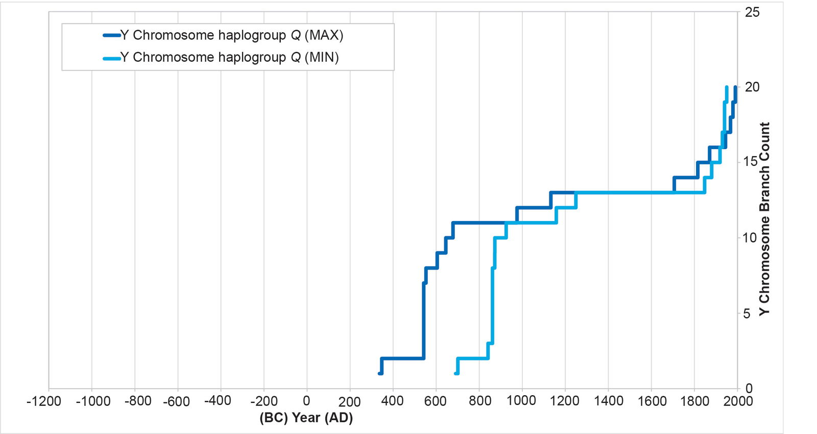
Fig. 1. History of population growth in Y chromosome haplogroup Q. The split between the Asian and American haplogroup Q branches occurred in the AD 300s to 600s. The population spike occurred in the AD 500s to 800s, followed eventually by a flat-lining of the curve that spanned the arrival of Europeans in AD 1492. Post-Contact, indigenous American populations recovered.
Initially, I attempted to replicate the Y chromosome Native American history with Native American mtDNA from haplogroups A, B, C, and D. The MIN and MAX values (see Methods for details on the calculations) for each mtDNA curve were extremely divergent from one another (figs. 2–5), with the mtDNA haplogroup D curve being the one exception. For all four haplogroups, the differences between the MIN and MAX curves were so large that they could have accommodated a population growth curve of almost any shape—rendering the results nearly meaningless (figs. 2–5).
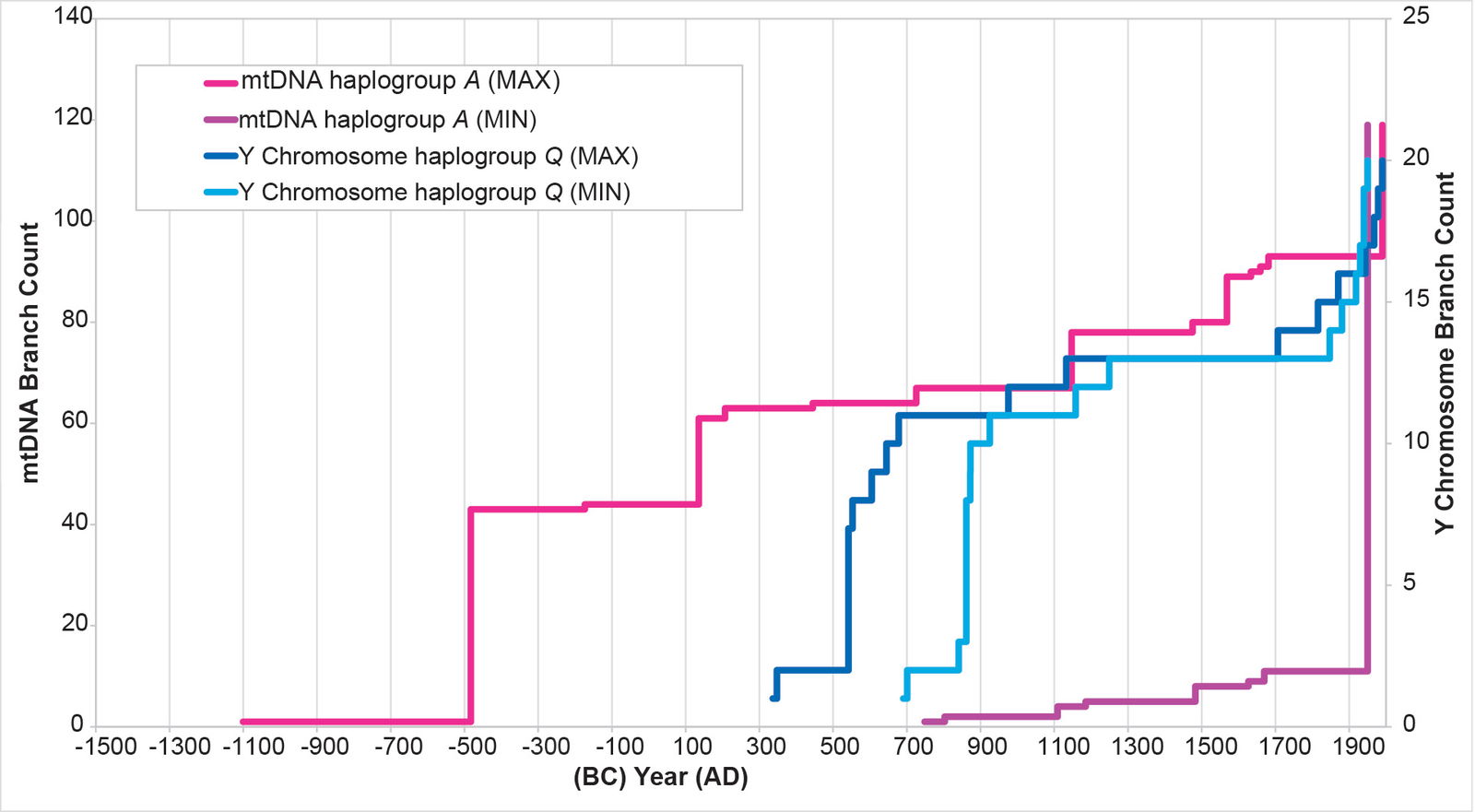
Fig. 2. History of population growth in mtDNA haplogroup A per the MIN/MAX method. The history of population growth in mtDNA haplogroup A was tested against the history in Y chromosome haplogroup Q. The MIN/MAX method for mtDNA haplogroup A produced results that were widely divergent from one another. They also had such a large range as to render them almost meaningless.
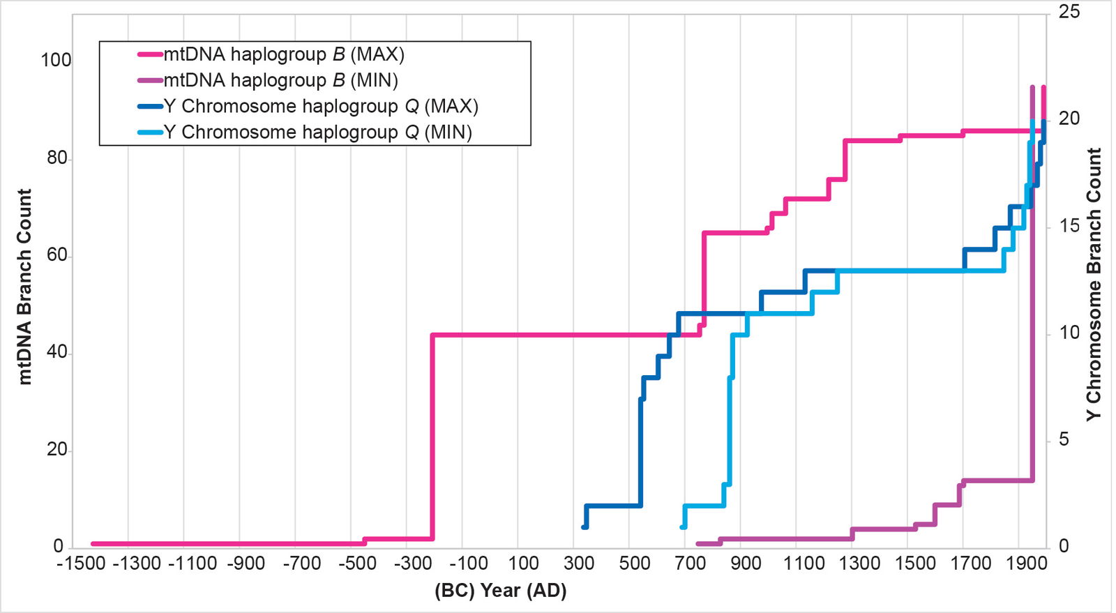
Fig. 3. History of population growth in mtDNA haplogroup B per the MIN/MAX method. The history of population growth in mtDNA haplogroup B was tested against the history in Y chromosome haplogroup Q. The MIN/MAX method for mtDNA haplogroup B produced results that were widely divergent from one another. They also had such a large range as to render them almost meaningless.
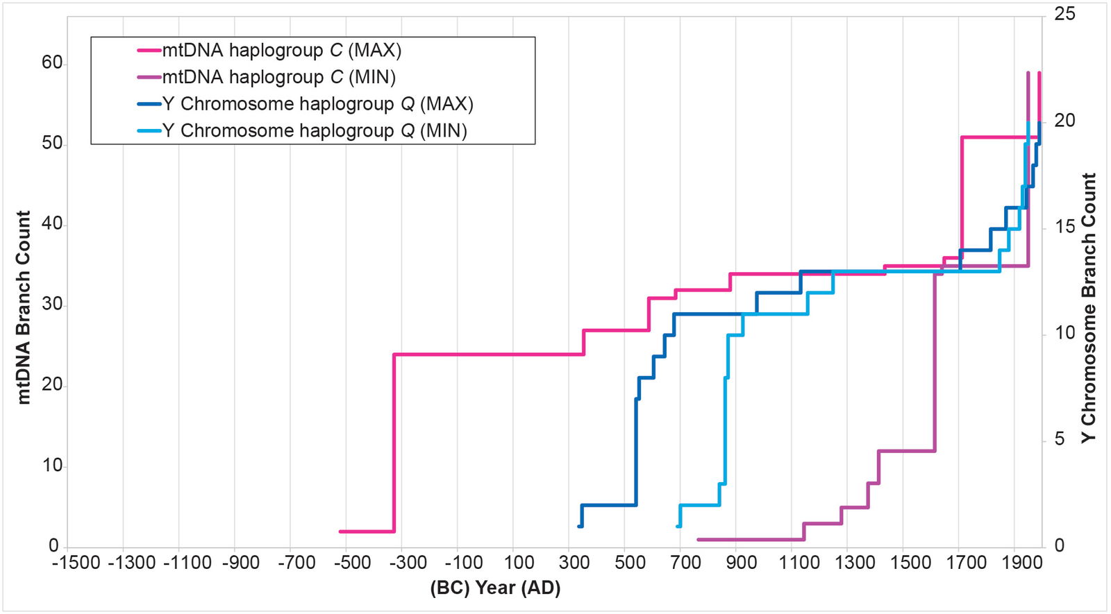
Fig. 4. History of population growth in mtDNA haplogroup C per the MIN/MAX method. The history of population growth in mtDNA haplogroup C was tested against the history in Y chromosome haplogroup Q. The MIN/MAX method for mtDNA haplogroup C produced results that were divergent from one another. They also had such a large range as to render them almost meaningless.
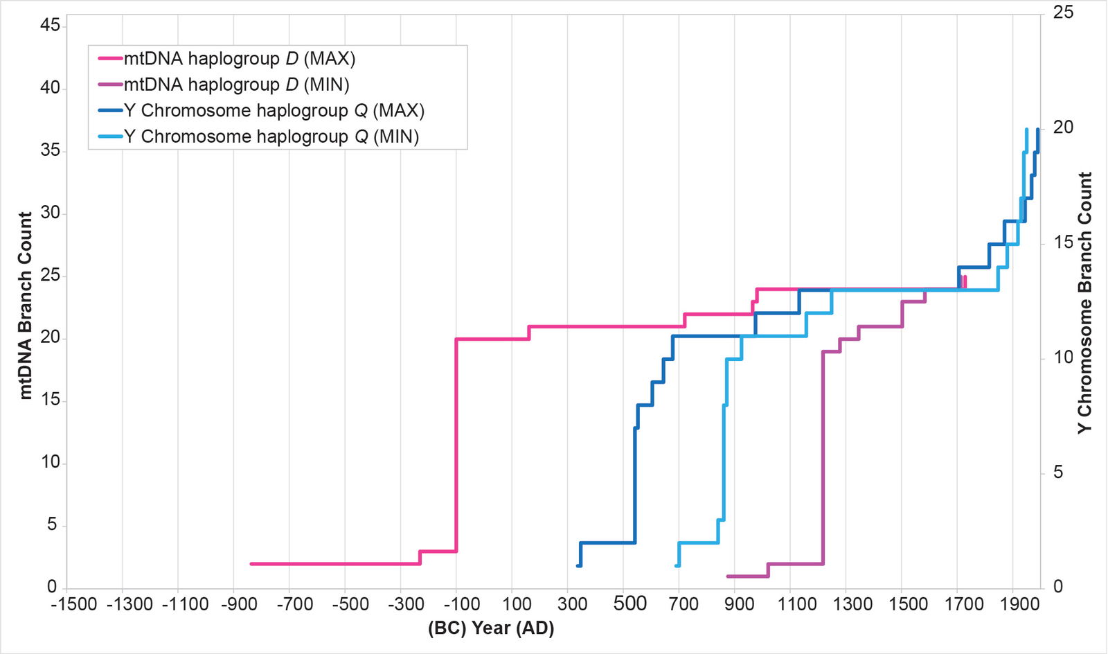
Fig. 5. History of population growth in mtDNA haplogroup D per the MIN/MAX method.The history of population growth in mtDNA haplogroup D was tested against the history in Y chromosome haplogroup Q. While the MIN/MAX method for mtDNA haplogroup D produced results that were somewhat mirrored, the results had such a large range as to render them almost meaningless.
Ultimately, the wide variance in these curves was a secondary consequence of the wide variance in mtDNA branch lengths.
Initially, I attempted to solve this problem by taking the average of the shortest and longest branch lengths. However, I found that this MIN/MAX AVG method (that is, not one described in the Methods section above) is easily skewed by outliers (data not shown). In addition, while some branch length clusters gave the appearance of being normally distributed (for example, see mtDNA haplogroup B in fig. 6), many others are one-tailed or have other odd shapes (for example, see the mtDNA haplogroup B subcluster in fig. 7). A simple MIN/MAX AVG method does not attempt to reflect the shapes of distributions like the latter.
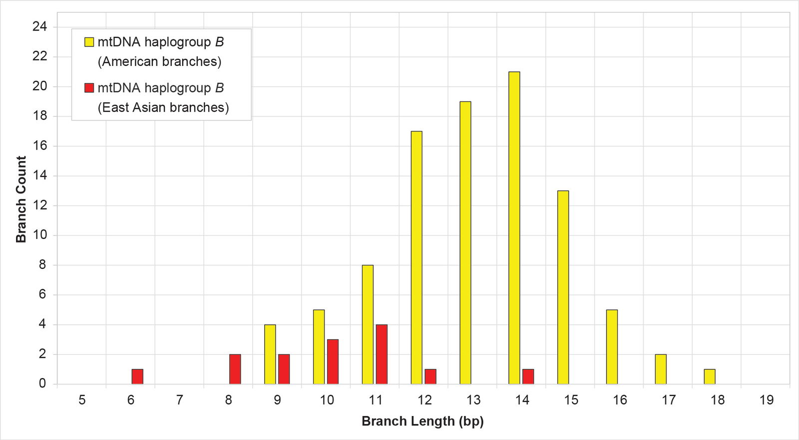
Fig. 6. Distribution of branch lengths in mtDNA haplogroup B. Branch lengths were grouped by geographic cluster. The American branches appeared to approximate a normal distribution.
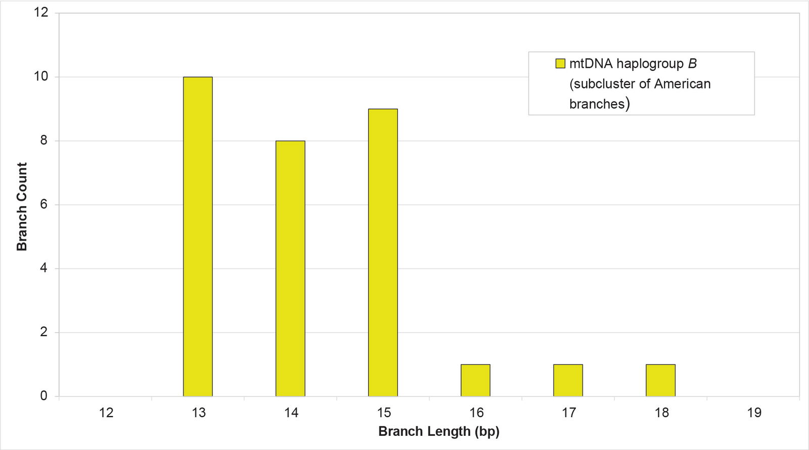
Fig. 7. Distribution of branch lengths in a subcluster of mtDNA haplogroup B. The branches did not appear to approximate a normal distribution. Rather, they looked significantly one-tailed.
In light of these concerns, I employed another version of this method. Instead of taking the average of the shortest and longest branch lengths in a cluster, I took the average of all the branch lengths in a cluster (“BL AVG method”; see Methods). In theory, this should reflect the shape of the branch length distribution to a degree. It should also be less affected by rare outliers.
The results of the BL AVG method produced a remarkable improvement in the agreement between mtDNA-based population growth curves and Y chromosome-based population growth curves (figs. 8–11). All four mtDNA haplogroup reconstructions showed a spike close to the Y chromosome range of A.D. 500s to 800s. Only the mtDNA haplogroup A spike fell outside the Y chromosome range—and this, just barely (fig. 8).
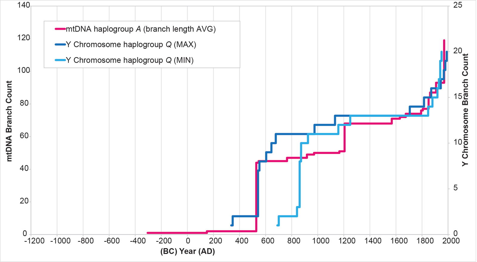
Fig. 8. History of population growth in mtDNA haplogroup A per the BL AVG method. The history of population growth in mtDNA haplogroup A was tested against the history in Y chromosome haplogroup Q, this time using the BL AVG method. The mtDNA results from the BL AVG method were a much better approximation of the Y chromosome history than the mtDNA results from the MIN/MAX method.
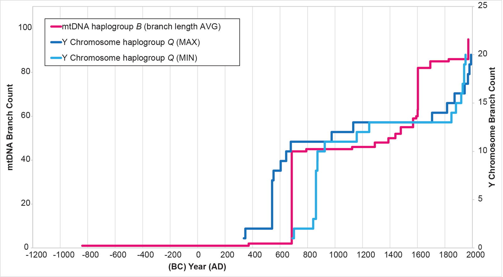
Fig. 9. History of population growth in mtDNA haplogroup B per the BL AVG method. The history of population growth in mtDNA haplogroup B was tested against the history in Y chromosome haplogroup Q, this time using the BL AVG method. The mtDNA results from the BL AVG method were a much better approximation of the Y chromosome history than the mtDNA results from the MIN/MAX method.
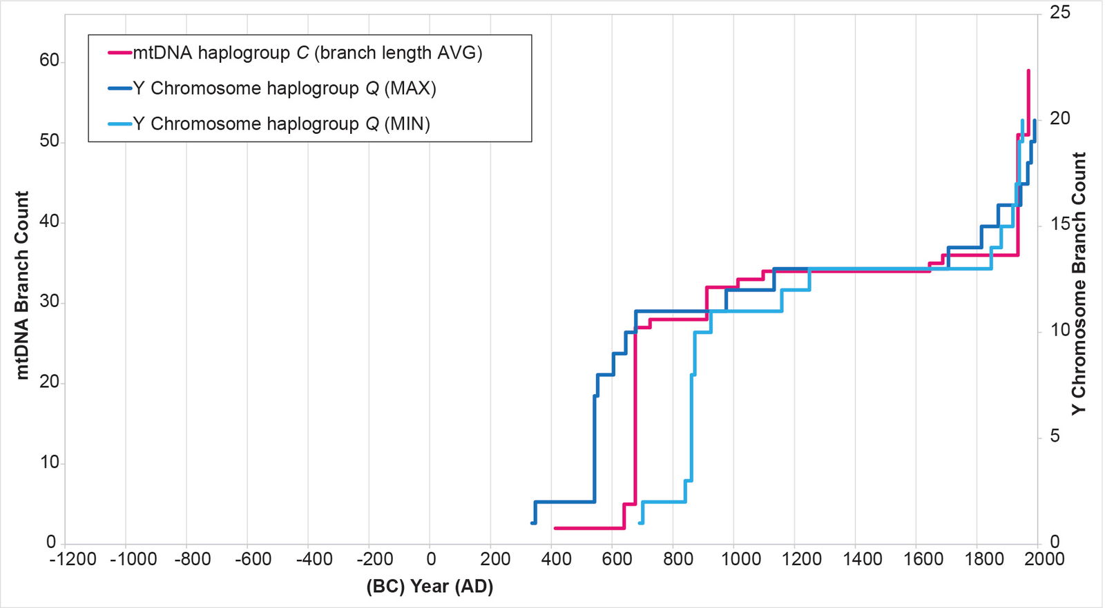
Fig. 10. History of population growth in mtDNA haplogroup C per the BL AVG method. The history of population growth in mtDNA haplogroup C was tested against the history in Y chromosome haplogroup Q, this time using the BL AVG method. The mtDNA results from the BL AVG method were a much better approximation of the Y chromosome history than the mtDNA results from the MIN/MAX method.
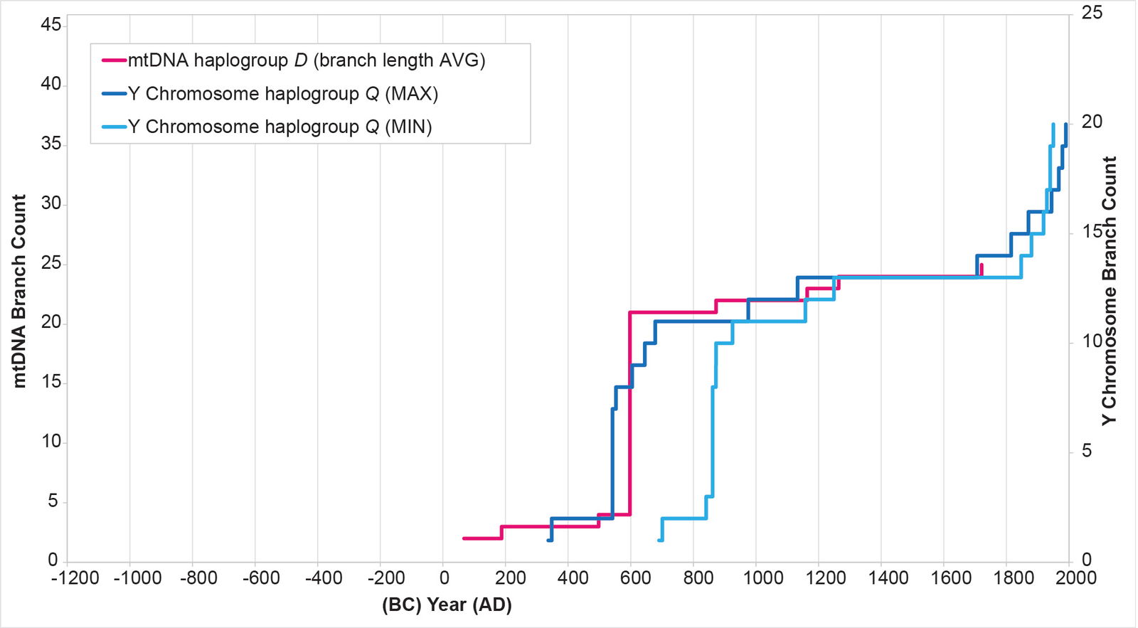
Fig. 11. History of population growth in mtDNA haplogroup D per the BL AVG method. The history of population growth in mtDNA haplogroup D was tested against the history in Y chromosome haplogroup Q, this time using the BL AVG method. The mtDNA results from the BL AVG method were a much better approximation of the Y chromosome history than the mtDNA results from the MIN/MAX method.
In section (A), I mentioned choosing an initial position for the 1 base pair branch at the base of the tree. I tested the alternative position—one where I shifted the relative position of the 1 base pair at the base of the tree (see Supplemental fig. 1 for original position). I changed the calculation such that the 1 base pair branch led to the section of the tree containing mtDNA haplogroups A and L and macrohaplogroup M, rather than to the section of the tree containing haplogroup B. This action brought mtDNA haplogroup A spike within the Y chromosome range (fig. 12) without driving the mtDNA haplogroup B spike outside of it (fig. 13). (The mtDNA haplogroup C and D spikes were unaffected by the root shift, due to how I calculate dates in this section of the tree; see Methods for details.)
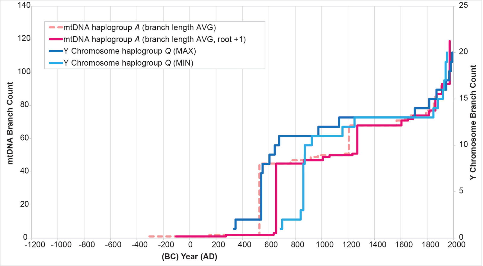
Fig. 12. History of population growth in mtDNA haplogroup A per the BL AVG method, but with a slight shift in root position. The history of population growth in mtDNA haplogroup A was tested against the history in Y chromosome haplogroup Q, this time using the BL AVG method and a slightly shifted root position. The mtDNA results from this method were an even better fit to the Y chromosome history than in the original (fig. 8).
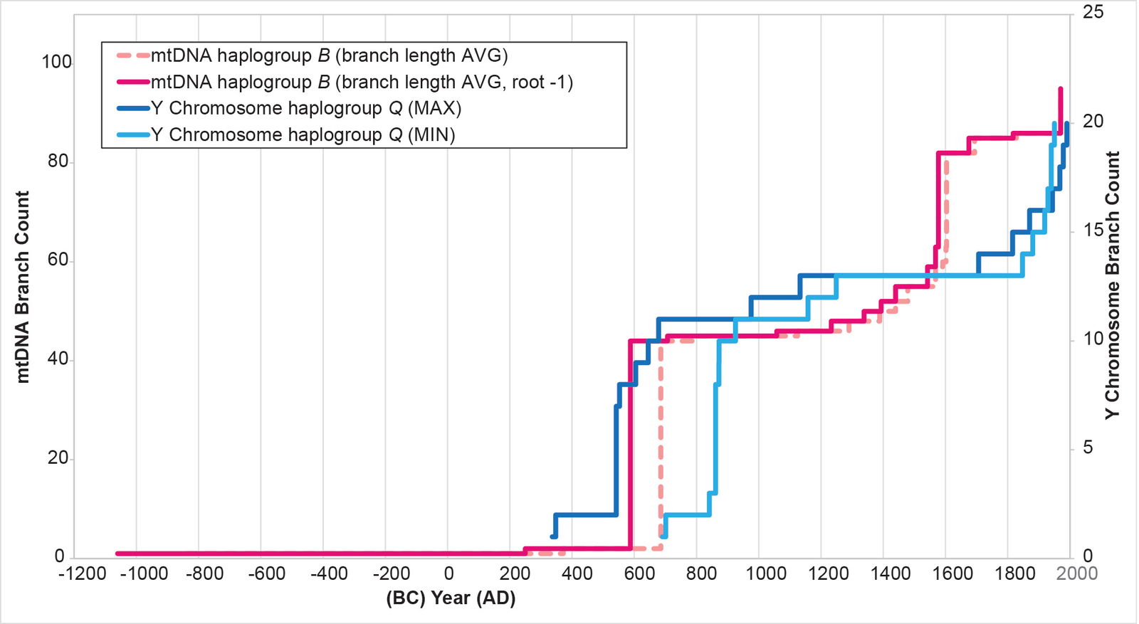
Fig. 13. History of population growth in mtDNA haplogroup B per the BL AVG method, but with a slight shift in root position. The history of population growth in mtDNA haplogroup B was tested against the history in Y chromosome haplogroup Q, this time using the BL AVG method and a slightly shifted root position. The mtDNA results from this method were as good as match as were the original (fig. 9).
In other parameters, the mtDNA haplogroup reconstructions differed in their ability to replicate the Y chromosome population reconstructions. For example, the mtDNA haplogroup C reconstruction showed tight alignment with the Y chromosome flat-lining and post-Contact population recovery (fig. 10). The mtDNA haplogroup D reconstruction showed tight alignment with the Y chromosome flat-lining, but little post-Contact population recovery (fig. 11). The mtDNA haplogroup A reconstruction showed strong alignment with the Y chromosome flat-lining and post-Contact population recovery (fig. 12). But between the initial spike and the subsequent flat-lining, the mtDNA haplogroup A reconstruction departed from the Y chromosome curve (fig. 12).
For mtDNA haplogroup B, the reconstruction showed flat-lining immediately after the initial spike. Then, where the Y chromosome curve showed flat-lining, the mtDNA curve showed growth (fig. 13).
To understand these discrepancies more deeply, I first observed that the population sampling strategies for the Y chromosome and mtDNA trees were different. The latter sampled several populations (CLM, MXL, PEL, PUR; see Methods) deeply (that is, 55 or more samples from each of the four populations). The Y chromosome tree was based on light sampling of more diverse populations—7 Pima from northwest Mexico, 2 Maya from the Mexican Yucatan, 2 Colombians, 5 Karitiana from Brazil, and 4 Surui from Brazil.
In light of these differences, I decomposed the mtDNA haplogroup-specific population reconstructions into population-specific growth curves—that is, curves for each of the CLM, MXL, PEL, and PUR populations. It was immediately clear that these four populations had different growth curves, both at the individual haplogroup level (for example, see the population-specific curves for mtDNA haplogroups A and B in figs. 14–15) and across all four haplogroups combined (figs. 16–19).
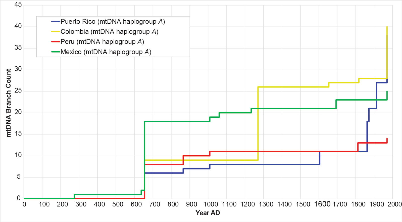
Fig. 14. History of population growth in mtDNA haplogroup A, but broken into population-specific curves. The history of population growth in mtDNA haplogroup A was tested against the history in Y chromosome haplogroup Q, this time decomposing the mtDNA haplogroup A curves by source population. Visually, the curves from each population were obviously different from one another.
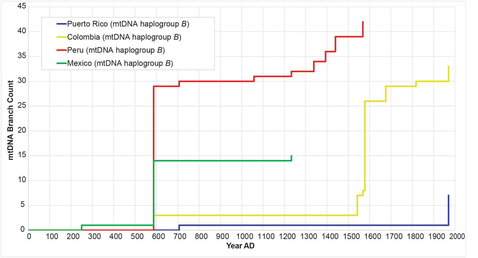
Fig. 15. History of population growth in mtDNA haplogroup B, but broken into population-specific curves. The history of population growth in mtDNA haplogroup B was tested against the history in Y chromosome haplogroup Q, this time decomposing the mtDNA haplogroup A curves by source population. Visually, the curves from each population were obviously different from one another.
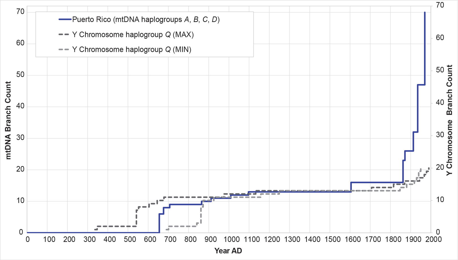
Fig. 16. History of population growth in the Puerto Rican population, across all four American mtDNA haplogroup clusters. The history of population growth in the Puerto Rican (PUR) population was tested against the history in Y chromosome haplogroup Q. The PUR population showed a strong match to the Y chromosome history, and an especially strong post-Contact spike.
Remarkably, all four populations mimicked the Y chromosome tree to one degree or another (figs. 16–19). The Puerto Rican curve captured the early population spike, the Contact-era flat-lining, and a robust post-Contact recovery (fig. 16). The Mexican and Peruvian curves both captured the early population spike and the Contact-era flat-lining (figs. 17–18). Neither showed much of any post-Contact population recovery. The Colombian curve resembled some of the other curves in that there were sections of flat-lining and sections of post-Contact recovery. But these sections were interrupted by population spikes, both in the AD 1200s and in the AD 1500s (fig. 19).
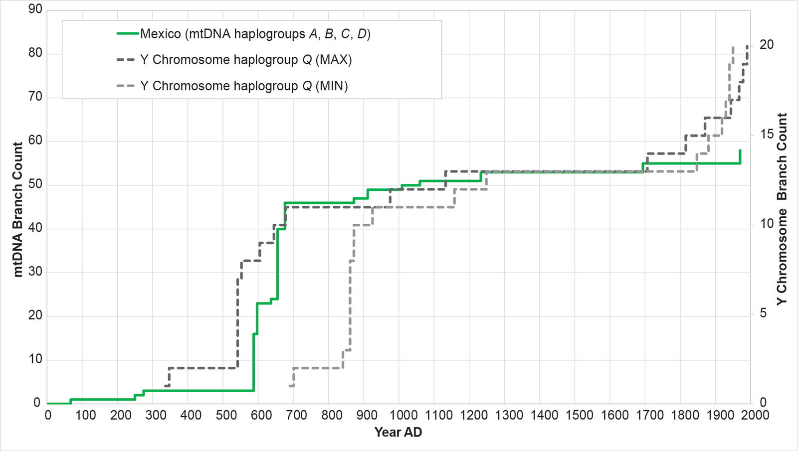
Fig. 17. History of population growth in the Mexican population, across all four American mtDNA haplogroup clusters. The history of population growth in the Mexican (MXL) population was tested against the history in Y chromosome haplogroup Q. The MXL population showed a strong match to the Y chromosome history, but very little post-Contact recovery.
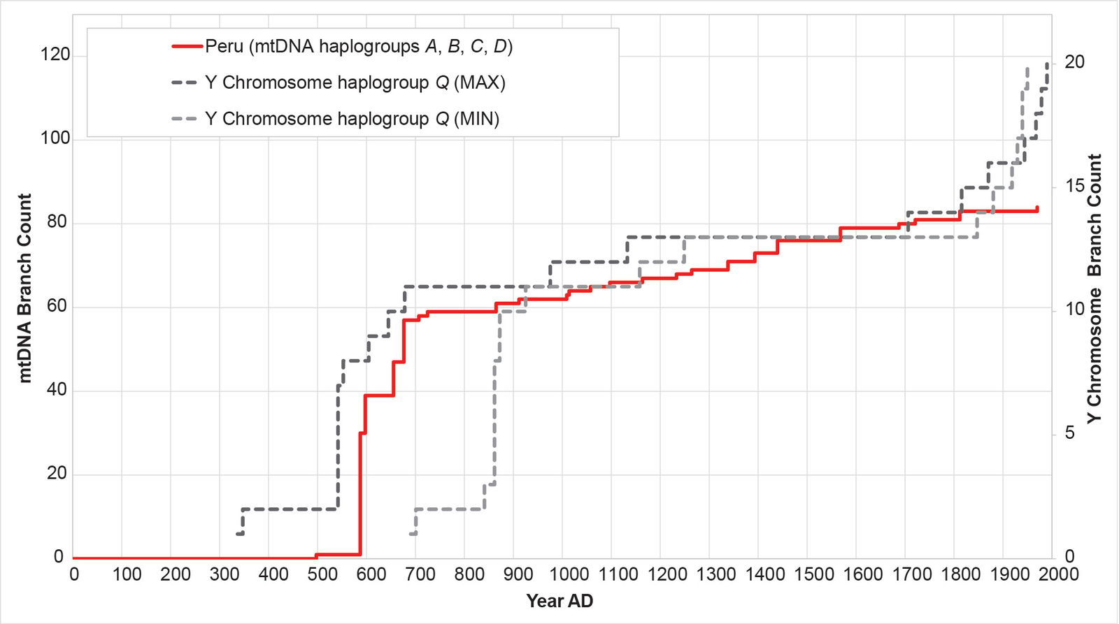
Fig. 18. History of population growth in the Peruvian population, across all four American mtDNA haplogroup clusters. The history of population growth in the Peruvian (PEL) population was tested against the history in Y chromosome haplogroup Q. The PEL population showed a strong match to the Y chromosome history, but very little post-Contact recovery.
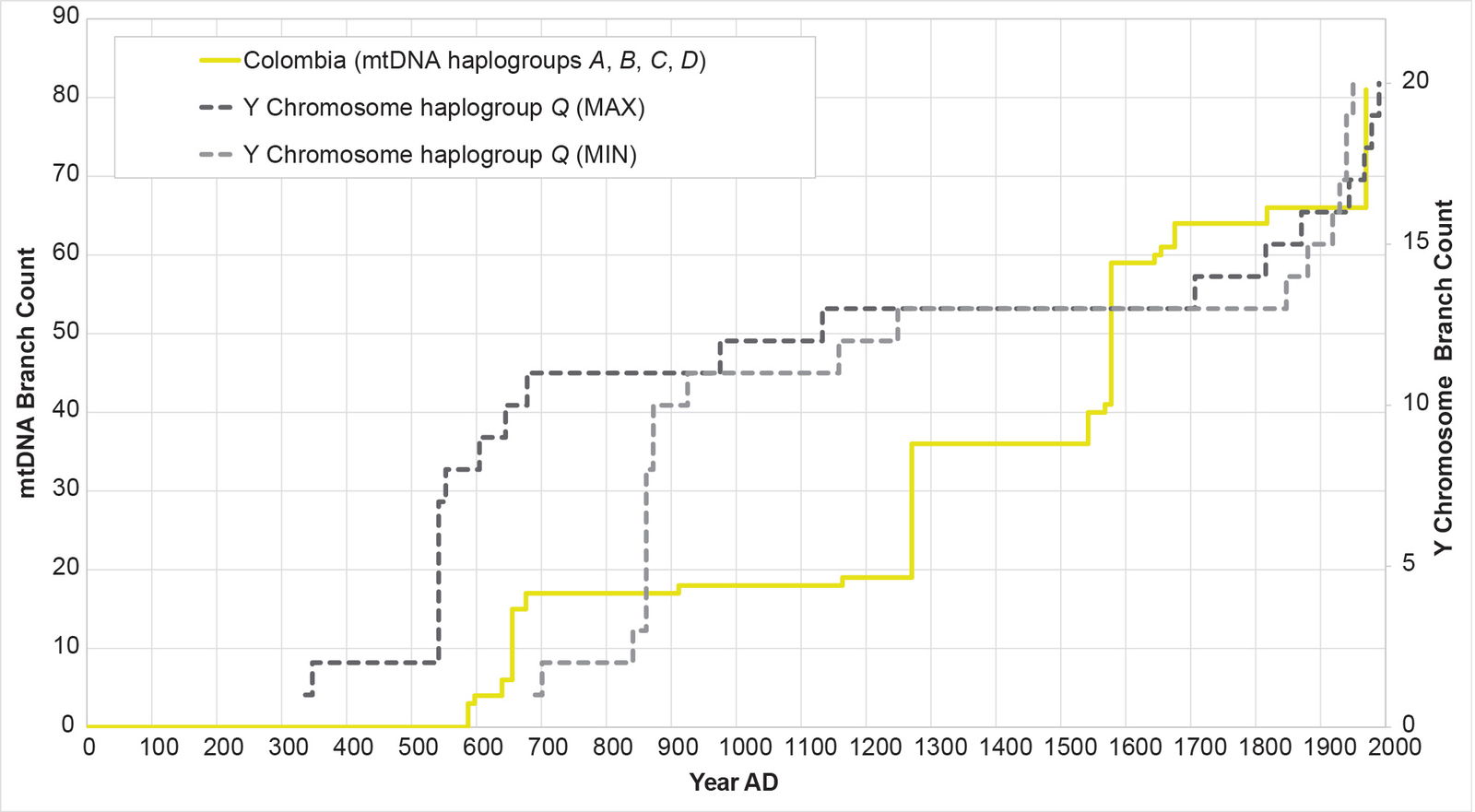
Fig. 19. History of population growth in the Colombian population, across all four American mtDNA haplogroup clusters. The history of population growth in the Colombian (CLM) population was tested against the history in Y chromosome haplogroup Q. The CLM population showed occasional match to the shape of the Y chromosome history, but these matches were interrupted by population spikes.
For the Colombian AD 1200s population spike, archaeology suggested an explanation. Pre-Columbian Colombia hosted the Muisca chiefdom. The archaeological sequence for the Muisca echoed the mtDNA-based population reconstructions:
Between circa 400 BC and AD 200 . . . known as the Herrera phase, population density was low . . . This changed in approximately AD 800–1200, during the Early Muisca phase, which was characterized by population growth (actually doubling in some regions) and increases in the size of communities . . . After AD 1200 until the arrival of the Spaniards circa AD 1600, the Late Muisca phase was marked by substantial population compared with the Early Muisca phase (estimated at between 170% and 300% growth).7
In the Colombian mtDNA population growth reconstruction, the branch count increased in AD 1270 from 19 to 36—a 189% increase.
In sum, once we decomposed each mtDNA haplogroup growth curve into the individual contributions from each source population, all four haplogroups showed strong agreement with the Y chromosome haplogroup Q curve, or with the archaeological history of population growth.
In fact, a deeper analysis of the post-Contact portion of each population-specific growth curve independently confirmed the accuracy of these reconstructions. For each of the four populations (or regions that they represent), the change in post-Contact census sizes is known. Each region experienced a population nadir, and then a recovery. The degree of recovery by AD 1875 differentiated these locations (table 2). The mtDNA population recoveries showed a remarkable correspondence to the known census population recoveries, with an R2 value of 0.95 (table 2).
Table 2. Post-Contact correlation in census and mtDNA population recoveries.
| Mexico | Caribbean | Colombia | Central Andes | |
| AD 1600 population (nadir) | 3,500,000 | 200,000 | 800,000 | 2,800,000 |
| AD 1875 population | 9,000,000 | 5,250,000 | 2,500,000 | 5,125,000 |
| Ratio: AD 1875/AD 1600 | 2.6 | 26.3 | 3.1 | 1.8 |
| Mexican (MXL) | Puerto Rican (PUR) | Colombian (CLM) | Peruvian (PEL) | |
| pre-AD 1492 branch count | 53 | 13 | 36 | 76 |
| total branch count | 58 | 70 | 81 | 84 |
| Ratio: Total/AD 1492 | 1.1 | 5.4 | 2.3 | 1.1 |
| R-squared for ratios | 0.95 | |||
As a final confirmation of these results, I compared populations-specific reconstructions for mtDNA and Y chromosome directly to one another. Practically, this is feasible for the Peruvian population only. In the 1000 Genomes Project Y chromosome tree, most of haplogroup Q branches are from the Peruvian population. The Peruvian mtDNA and Y chromosome curves show strong correspondence to one another (fig. 20).
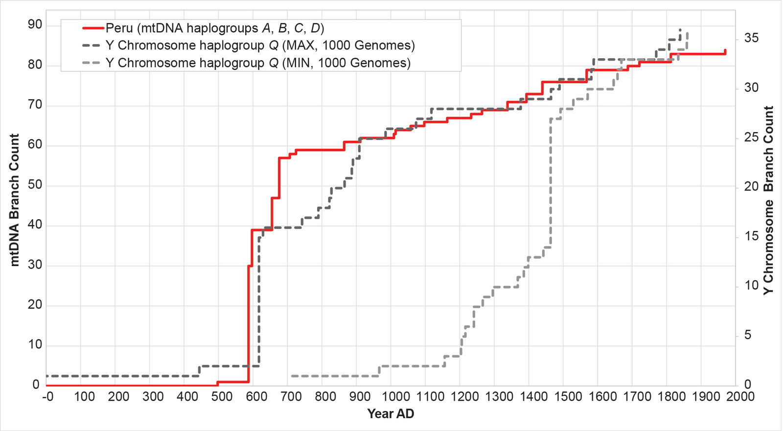
Fig. 20. The mtDNA and Y chromosome population histories for Peru show the same shape. The mtDNA history for the Peruvian (PEL) population was reconstructed with the BL AVG method. The Y chromosome history for the PEL population was reconstructed with the MIN/MAX method. The MAX Y chromosome curve showed significant overlap with the BL AVG mtDNA curve.
Thus, though the initial mtDNA haplogroup-specific reconstructions showed some differences from the Y chromosome reconstructions, the explanation was clear: Population-specific differences in growth and recovery. Furthermore, these results demonstrated that the mtDNA tree and the BL AVG method was exquisitely sensitive to the known history of American population growth.
The BL AVG method manifested the existence of a real mtDNA clock.
C. At least one BC-era migration from Asia into the Americas
In the Y chromosome tree, the most recent migration from Asia into the Americas happened around AD 900. The most consequential, in the AD 300s to 600s.
In the mtDNA tree, none of the four haplogroups arrived in the Americas around AD 900.8 But two seemed to mirror the Y chromosome migration in the AD 300s to 600s.
Specifically, the American and Asian branches in mtDNA haplogroup C separated in the AD 600s (table 3; see Supplemental table 4 for details of the calculations). One tiny cluster of one American and one Asian branch in haplogroup C seemed initially to separate later (see node 3463 in Supplemental fig. 1). But this may have been an artifact of the dataset, as addition of a close relative bumped the link back (see node 3563 in Supplemental fig. 2).
Also, for the main haplogroup D cluster of American branches, the initial calculations put the origin of the main cluster in the early AD era—that is, close to the time of Y chromosome haplogroup Q arrival (see Supplemental table 4 for details of the calculations). These initial calculations also put the main spike near the low end of the Y chromosome range (fig. 11). I recalculated the BL AVG method for haplogroup D, this time adding (±) 0.5 of a standard deviation to the math. The (–) 0.5 standard deviation calculation put the population spike at the higher end of the Y chromosome range (fig. 21). It also put the time of origin for the main American haplogroup D cluster around AD 300. When I calculated this date using just the American branches to determine the BL AVG, the date jumped to AD 466—well within the time of origin range for the Native American cluster in Y chromosome haplogroup Q (table 3).
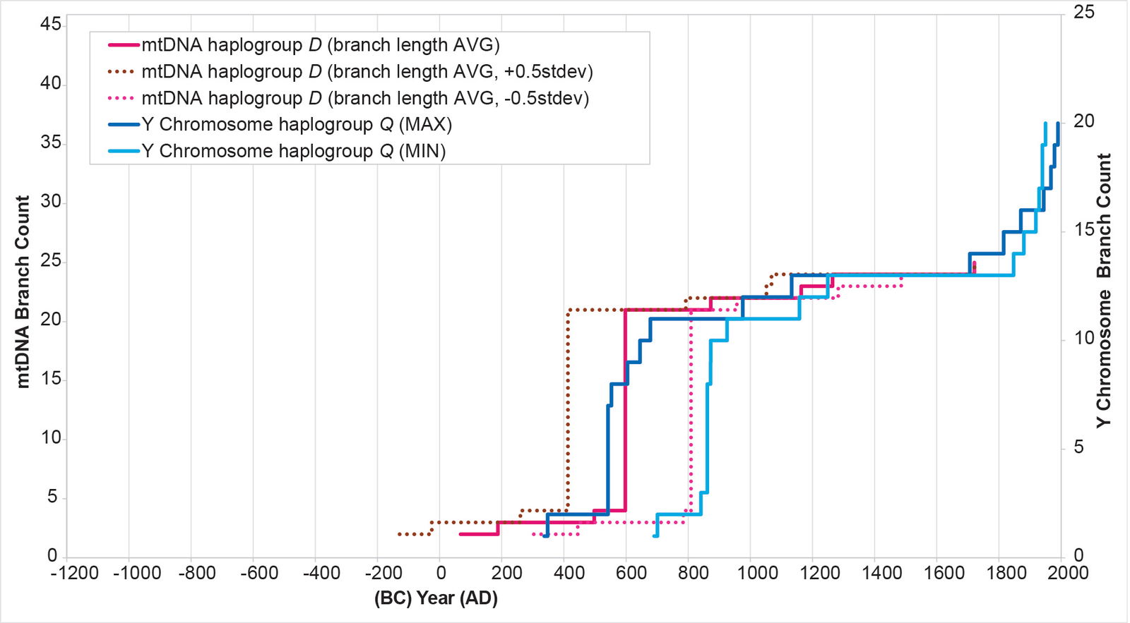
Fig. 21. History of population growth in mtDNA haplogroup D per the BL AVG method, but with standard deviation calculations. The history of population growth in mtDNA haplogroup D was tested against the history in Y chromosome haplogroup Q, this time using the BL AVG method and (±) 0.5 of standard deviation of the BL AVG. The BL AVG and the BL AVG (–) 0.5 of the standard deviation fit the range of the Y chromosome spike in the AD 500s to 800s.
Table 3. Summary of time of origin for American mtDNA clusters.
| mtDNA haplogroup |
American cluster: Time of origin |
Y Chromosome haplogroup equivalent |
| A | 181 BC to AD 46? | (none this early) |
| B | 1060 to 932 BC | (none this early) |
| C | AD 676 | Q |
| D | AD 466 | Q |
Thus, both mtDNA haplogroup C and mtDNA haplogroup D seemed to document a migration equivalent to the one recorded by Y chromosome haplogroup Q.
For mtDNA haplogroup A, at face value, the American branches separated from the Asian ones in 104 BC. Using the full spectrum of dates derived from using the standard deviation (fig. 22; for methodological details, see Supplemental table 4), the range was 181 BC to AD 46. This was clearly before the arrival of Y chromosome haplogroup Q in the Americas.
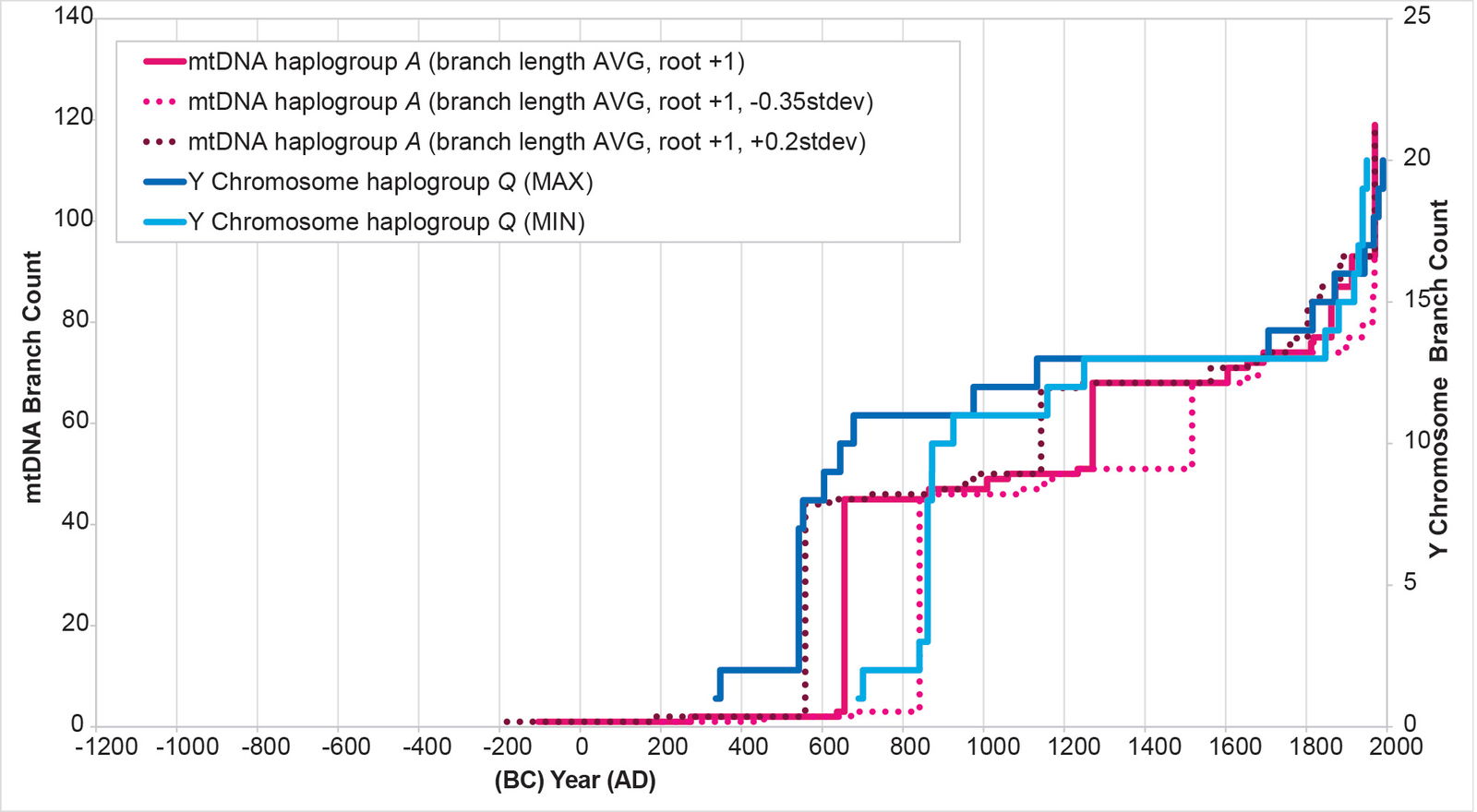
Fig. 22. History of population growth in mtDNA haplogroup A per the BL AVG method, but with standard deviation calculations. The history of population growth in mtDNA haplogroup A was tested against the history in Y chromosome haplogroup Q, this time using the BL AVG method, the slightly shifted root position, and (+) 0.2 and (–) 0.35 of standard deviation of the BL AVG. The standard deviations were empirically tested until a value was found that spanned the range of Y chromosome spike dates.
But the YFULL database9 listed a single Japanese individual10 as part of the main American population spike. My own analysis confirmed its late placement in the American part of the haplogroup A tree (see Supplemental fig. 2). This would suggest a separation between Asian and American branches in the AD 600s, making mtDNA haplogroup A an equivalent to Y chromosome haplogroup Q.
Did mtDNA haplogroup A arrive in the Americas as a contemporary of Y chromosome haplogroup Q? Several considerations suggested that the original BC date of separation may have been correct. First, the YFULL Japanese branch was rare. By my own estimates, its frequency was less than 1 in 1200 Japanese individuals (data not shown).
Second, based on the data in the YFULL database for mtDNA haplogroups A, B, C, and D, mtDNA haplogroup A was especially enriched in Arctic samples as compared to the other haplogroups (see also Lorenz and Smith 1996, and Kumar et al. 2011). I wondered if the Japanese individual represented, not an indigenous Japanese lineage, but rather spillover from the Arctic populations.
Third, the original time of separation—104 BC—was, apparently, a time of rapid population growth and/or population dispersal in East Asia. When I reconstructed the population history for the East Asian branches in mtDNA haplogroup A, this conclusion emerged (fig. 23; see Supplemental table 4 for details of the calculations). Thus, if East Asians were already on the move, then conditions may have been ripe for a migration to the Americas.
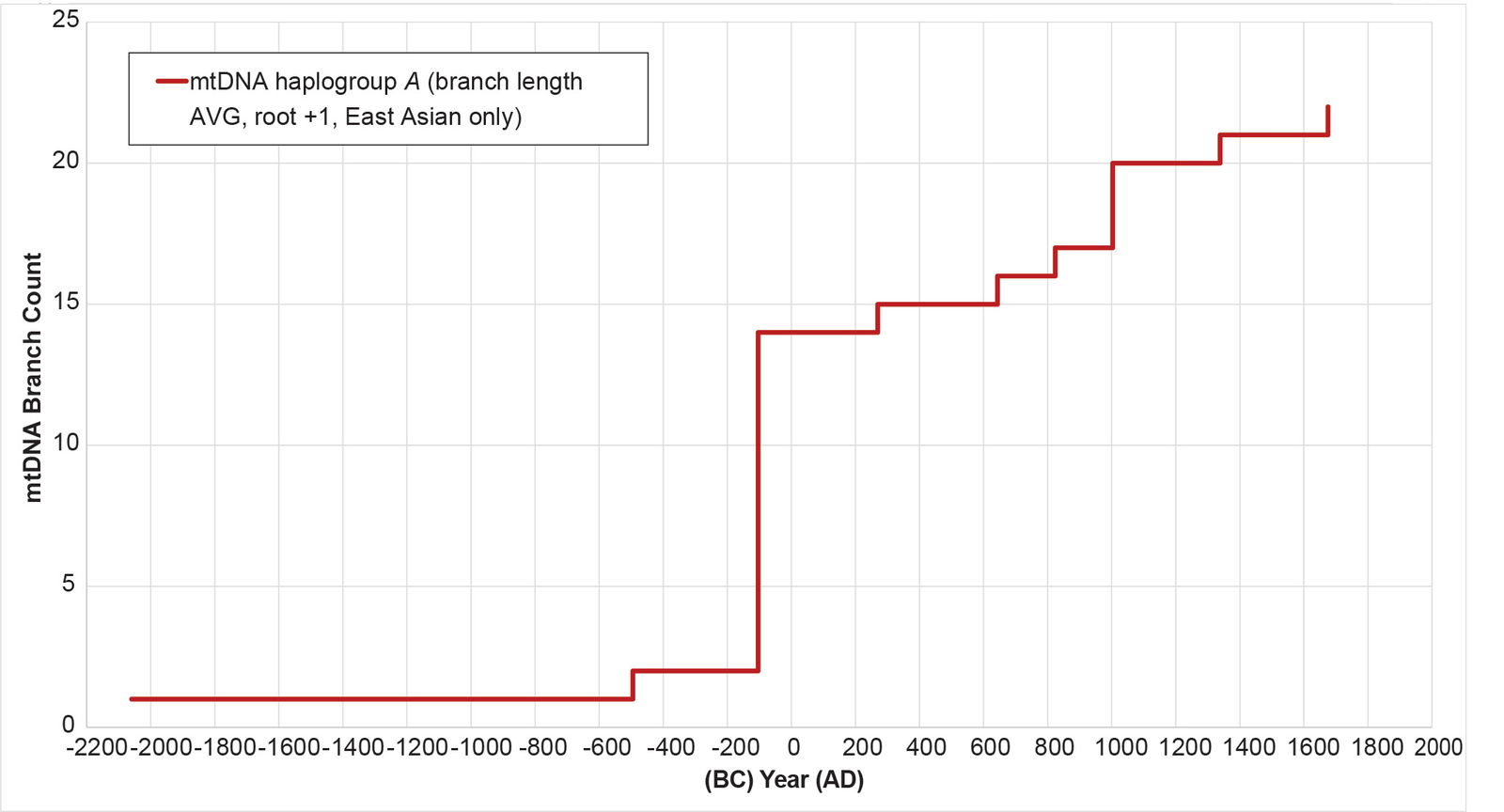
Fig. 23. History of population growth in mtDNA haplogroup A per the BL AVG method, but in the East Asian sister branches. The history of population growth in mtDNA haplogroup A East Asian branches was reconstructed using the BL AVG method. The resultant curve showed a population spike and/or dispersal around 100 BC.
Fourth, the known historical context for Central and East Asia in the last century BC was similar to the context during later Y chromosome migrations. When Y chromosome haplogroup Q arrived in the Americas, Central Asia was experiencing the Völkerwanderung. The Huns invaded Europe, and the Xianbei took over northern China. No surprise, then, that during this period a third Central Asian population migrated to the Americas. When Y chromosome haplogroup C arrived in the Americas several centuries later, the Magyars and Central Asian Turkic peoples were headed towards Europe. Again, it’s no shock that another Central Asian people group migrated during this time to the Americas. In the last century BC, the putative time of migration of mtDNA haplogroup A into the Americas, Central/northeast Asia was again alive with activity.
Specifically, from 209 BC to 49 BC, one of the more famous Central Asian/Mongolian peoples—the Xiongnu—rose and fell (Yü 1990; Beckwith 2009). To be sure, there were other militaristic neighbors of the Xiongnu during this era—Yueh-chih among others (Beckwith 2009; Yü 1990). Clashes between the Xiongnu and their Central Asian/Mongolian neighbors promoted migrations during this period (Beckwith 2009; Yü 1990). But it was the Xiongnu who broke up right around the time that mtDNA haplogroup A left Asia for the Americas (Beckwith 2009; Yü 1990). It’s plausible that Xiongnu refugees escaped to the Americas—or that the surviving Xiongnu simply picked up roots and sought military success elsewhere (that is, the Americas) rather than in China.
The details of the East Asian cluster of mtDNA haplogroup A suggested a narrative consistent with these inferences. Before the population spike in 104 BC (fig. 23), the East Asian branches were preceded by a long 4 base pair flat line (fig. 24). Almost by definition from the methods derived in Jeanson (2019) and Jeanson (2022), this would imply a historically small population size. Historically large population sizes were found inside China; small population sizes, outside China to the north and west into Central Asia (McEvedy and Jones 1978), where the Xiongnu made their home.
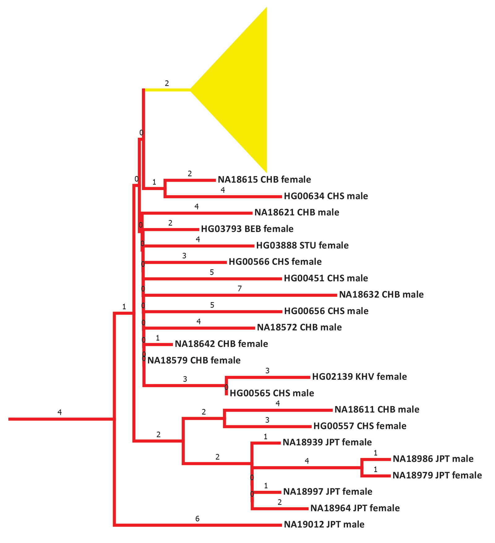
Fig. 24. Details of the early section of the mtDNA haplogroup A branches. Primarily East Asian branches and/or clusters were colored in red. The individual Native American branches after the flat 2 base pair line were collapsed into a single triangle and colored in yellow. Base pairs are shown above the branches.
Also, before the population spike in 104 BC (fig. 23), the East Asian branches experienced a single branching event (figs. 23–24), around 495 BC (see Supplemental table 4 for details of the calculations). Evidence for a significant Central Asian presence in Mongolia/northeastern Asia first appears in the 700s to 600s BC (Beckwith 2009). In the 600s to 500s, the Chinese invaded the Mongolian/northeastern Asian region (Beckwith 2009). The Chinese first built walls against these northern invaders in the 300s BC (Yü 1990). Perhaps this historical sequence of events prompted a branching event in 495 BC, in the lands from which the Xiongnu would eventually spring a few centuries later.
Fifth, the archaeological context for the Americas in the last century BC suggested a plausible and intriguing cause-effect relationship for the arrival of mtDNA haplogroup A. Consider: If we take the origin of mtDNA haplogroup A as 181 BC to AD 46, this is definitely before the arrival of Y chromosome haplogroup Q. Yet the arrival of the latter apparently wiped out the earlier indigenous American Y chromosome lineages. Presumably, for the early indigenous mtDNA lineages to survive the Y chromosome haplogroup Q invasion, they would have needed to have been part of a large, pre-invasion population size. That is, statistically, the greater the pre-invasion population size, the greater the chances that a lineage would have survived.
Which American regions concentrated people prior to the arrival of Y chromosome haplogroup Q? To be sure, the lowland Preclassic Maya erected a massive civilization, which would have required a large number of man hours to construct (Hansen et al. 2023). But when Y chromosome haplogroup Q invaded, one of the biggest cities was Teotihuacan in central Mexico. Upper estimates place the population size at 200,000 people (Coe and Koontz 2013). Right around the time (Coe and Koontz 2013) that Y chromosome haplogroup Q arrived, Teotihuacan was violently overthrown, and its population dramatically collapsed (Gorenflo, Robertson, and Nichols 2024). This was just a few centuries removed from Teotihuacan’s rapid population rise—when it “grew from almost nothing to become a large city” (Cowgill 2015, 53) in the 100s BC (Cowgill 2015; Gorenflo, Robertson, and Nichols 2024).
The American branches of mtDNA haplogroup A fit this history of Teotihuacan. Again, the timing of the arrival of mtDNA haplogroup A was just in time to contribute to Teotihuacan’s growth “from almost nothing to become a large city” (Cowgill 2015, 53). But the post-arrival events also fit the history of Teotihuacan. After the split from the East Asian cluster, the American mtDNA haplogroup A showed a flat 2 base pair line (fig. 24; see also Supplemental fig. 1). This indicated no population growth or a population collapse—perhaps the collapse that the arrival of Y chromosome haplogroup Q seems to have induced.
In sum, multiple lines of evidence suggested that mtDNA haplogroup A was brought to the Americas from Asia—perhaps by relatives of the Xiongnu—in the last 1–2 centuries BC (table 3), and that this lineage may have spawned the metropolis at Teotihuacan.
This conclusion rests on the fact that I analyzed strictly the coding region of mtDNA, and not the D-loop. The mainstream definition for American mtDNA haplogroup A included 6 to 7 mutational steps from the Asian cluster to the American cluster (see definition for mtDNA haplogroup A2 in the YFULL database11 and in Kumar et al. 2011). The majority of the mainstream mutational steps were in the D-loop. Had I included D-loop sequences, my mtDNA correlations to the history of Teotihuacan likely would have disappeared. But not because the D-loop sequences would have pushed the origin date forward in time to the arrival of Y chromosome haplogroup Q. Rather, the time of origin would likely have been bumped back deeper into the BC era.
In other words, under this scenario, mtDNA haplogroup A would still have represented one of the deep lineages that has been missing from the Y chromosome analysis of the Americas.
Again, the rare Japanese branch in the main mtDNA haplogroup A population spike left a lingering asterisk by these conclusions. If this doubt can be resolved, the resultant narrative from mtDNA haplogroup A would be compelling.
For mtDNA haplogroup B, the time of origin for the American branches was deep in the first millennium BC. The initial results showed a date of 1060 BC (table 3). But I noticed that these initial calculations put the main population spike near the low end of the Y chromosome range (fig. 13). I recalculated the BL AVG method for haplogroup B, this time adding (±) 0.5 of a standard deviation to the math. The (–) 0.5 standard deviation calculation put the population spike at the higher end of the Y chromosome range (fig. 25). It also put the time of origin for the main American haplogroup B cluster at 932 BC (table 3).
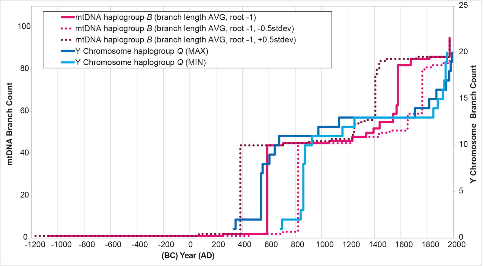
Fig. 25. History of population growth in mtDNA haplogroup B per the BL AVG method, but with standard deviation calculations. The history of population growth in mtDNA haplogroup B was tested against the history in Y chromosome haplogroup Q, this time using the BL AVG method and (±) 0.5 of standard deviation of the BL AVG. The BL AVG and the BL AVG (–) 0.5 of the standard deviation fit the range of the Y chromosome spike in the AD 500s to 800s.
In visual terms, this very early split time was driven by a long flat 4 base pair branch that connected the American cluster to the Asian cluster (fig. 26; see also Supplemental fig. 1). In the mainstream mtDNA models, 5 mutational steps linked the American and Asian clusters (see the YFULL database12 and Kumar et al. 2011). Unlike mtDNA haplogroup A, the mtDNA haplogroup B mutational steps were all in the coding region, not the D-loop. Also unlike mtDNA haplogroup A, the mtDNA haplogroup B American cluster had no rare Japanese individual. It also had little Arctic presence (see YFULL database,13 Lorenz and Smith 1996, and Kumar et al. 2011).
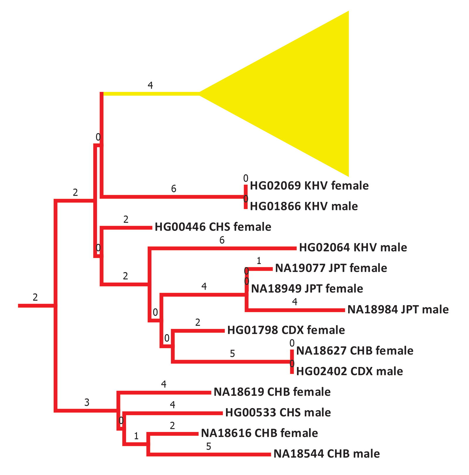
Fig. 26. Details of the early section of the mtDNA haplogroup B branches. Primarily East Asian branches and/or clusters were colored in red. The individual Native American branches after the flat 4 base pair line were collapsed into a single triangle and colored in yellow. Base pairs are shown above the branches.
Was this 4 base pair connector a reflection of the residence of mtDNA haplogroup B in America? Or, to put it more bluntly, how do we know that future investigations are not going to identify Asian branches in the middle of this cluster? In short, we don’t know. Current databases with Central and East Asian samples show no branches in this region (that is, see the YFULL database14 and Askapuli et al. 2022). But future studies could change this scenario.
Nevertheless, several considerations suggested that the ancient origin of American mtDNA haplogroup B was real. First, an analogy to the Y chromosome tree planted the mtDNA migration in a time of significant Y chromosome migratory activity. Within East Asia, 1000 BC saw the origin of the major haplogroup O subgroups, which eventually ended up all over East and Southeast Asia (Jeanson 2022). In Central Asia, the Q and R haplogroups separated around 1000 BC (Jeanson 2022). Y chromosome haplogroup D split into its Tibetan, Japanese, and Great Andamanese branches around this time (Jeanson 2022). Finally, around 1000 BC, Y chromosome haplogroup C left Siberia for Japan, and then traveled into island Southeast Asia where a subgroup broke away for South Asia (Jeanson 2022). Around the 1000s to 700s 1000 BC, the remaining population in island Southeast Asia broke east into the Pacific (Jeanson 2022).
In terms of timing the American origin of mtDNA haplogroup B is exactly contemporary with these Y chromosome events (table 3). Given the direction of the Y chromosome haplogroup C migration—east out of Siberia—it is plausible that one subpopulation might have gone north and east into the Americas while the rest went south into Japan and eventually east into the Pacific.
Second, a sister branch to the American mtDNA haplogroup B underscored these conclusions. Today, mtDNA haplogroup B is the dominant Polynesian branch (Benton et al. 2012; Hudjashov et al. 2018; Kim et al. 2012). A cluster of Pacific mtDNA haplogroup B sequences sits near the American mtDNA haplogroup B branches (see Supplemental fig. 2). I calculated the time of origin for the separation of this Pacific cluster from the Asian cluster. The BL AVG method put the date at 768 BC (see Supplemental table 5 for details on the calculations).
When I reconstructed the population history for this Pacific cluster, it initially showed a population spike/dispersal around AD 1400 (fig. 27). The individuals in the cluster include both Melanesians and Polynesians like Cook Islanders (see Supplemental fig. 2). Archaeology suggests that the most distant Polynesian islands—Hawaii, New Zealand, Rapa Nui—were colonized perhaps a few centuries earlier (Kirch 2017; Wilmshurst et al. 2011). So I recalculated the BL AVG method for Pacific haplogroup B, this time adding (±) 0.5 of a standard deviation to the math. The (+) 0.5 standard deviation calculation put the population spike/dispersal into the AD 1100s, which might be a more accurate reflection of Pacific history (fig. 27). It also put the split in the Asian and Pacific clusters at 875 B.C. (see Supplemental table 5 for details on the calculations).
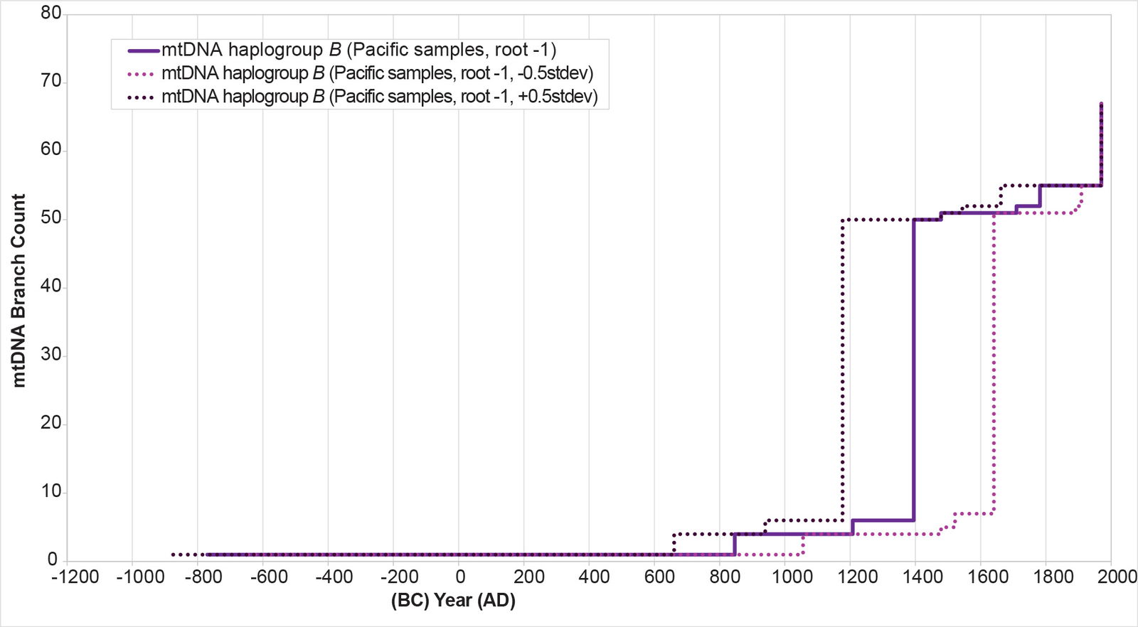
Fig. 27. History of population growth in the Pacific cluster of mtDNA haplogroup B per the BL AVG method and standard deviation calculations. The history of population growth the Pacific cluster of mtDNA haplogroup B was reconstructed using the BL AVG method and (±) 0.5 of standard deviation of the BL AVG. The BL AVG (+) 0.5 of the standard deviation brought the population spike/dispersal period from approximately AD 1400s (BL AVG without standard deviation) back into the AD 1100s, which might be a better fit to the archaeological history of the Pacific.
These origins dates fall within the range of the ancient Y chromosome haplogroup C migration, particularly the range for when haplogroup C made the final move east into the Pacific (see above; see also Jeanson 2022 for more detailed justification for Y chromosome dates).
Thus, mtDNA haplogroup B seemed to be the equivalent of the ancient Y chromosome haplogroup C migration.
Third, in the Americas, the late first millennium BC was a time of significant transition.
During the tenth century BC, both in the Central and Northern Maya Areas, we now have, for the first time, substantial evidence for a Maya population.15
These nascent populations precipitated even bigger change in the centuries following:
As communities linked to Olmec ideas went into steep decline c. 400 BC, rapid changes took place in the Maya area. The timing cannot be coincidental, but its meaning is unclear. What we do know is that, as populations rose, the southern lowlands of the peninsula became a new hotbed for complexity in Mesoamerica, resulting in the construction of immense cities, particularly in the Peten’s so-called Mirador Basin . . . Concurrently, we see in this epoch the beginnings of Maya hieroglyphic writing and the calendar.16
In other words, mtDNA haplogroup B seemed to have arrived in the Americas just as the Mayan civilization was rising—a timing that seemed oddly coincidental.
Fourth, this Mayan context provided a ready explanation for the flat 4 base pair line in mtDNA haplogroup B. If this line did indeed echo the history of population growth in mtDNA haplogroup B, then it must have represented a period of population stasis or collapse—almost by definition, as per the methods developed in Jeanson (2019) and Jeanson (2022) for the Y chromosome.
In the Mayan area, this inference found a ready archaeological echo:
By c. AD 150, the Mirador Basin cities had suffered a collapse as disastrous as that which would occur throughout the southern lowlands at the end of the Classic.17
Thus, mtDNA haplogroup B suggested itself as a strong candidate for the origin of the Mayan peoples and for one of the “missing lineages” in the YEC model for pre-Columbian American history.
D. Sex-specific lineage survival
These findings raised another question: Why did one (or more) mtDNA lineages from the B.C. era persist, but Y chromosome lineages were lost? The Post-Contact history of the Americas suggested an answer.
In the post-Contact era, sex-selective population change happened. Each of the four 1000 Genomes Populations today have a higher percentage of indigenous mtDNA lineages than Y chromosome lineages. For example, only 5% to 7% of Colombian and Puerto Rican males belong to an indigenous Y chromosome lineage (see Supplemental table 2 for justification). Yet, in terms of mtDNA, 88% of Colombians and 70% of Puerto Ricans belong to indigenous lineages (table 4; see Supplemental table 3 for justification). Thirty percent of Mexican males belong to indigenous Y chromosome lineages (see Supplemental table 2 for justification); 85% of Mexicans belong to indigenous mtDNA lineages (table 4; see Supplemental table 3 for justification). For Peruvians, 61% of Y chromosome lineages are indigenous; for mtDNA, the number reaches almost 100% (table 4; see Supplemental table 3 for justification). Thus, when Europeans arrived in the Americas, they seemed to have preferentially diminished or replaced the male Y chromosome lineages, but left the female mtDNA lineages intact.
A similar phenomenon seemed to have occurred in the pre-Contact era. Specifically, to date, no pre-AD 300s Y chromosome lineages have been discovered in the Americas. In other words, all extant indigenous Y chromosomes arrived in the Americas in the AD era. None of the extant Y chromosome lineages linked modern populations back to the BC era. Yet, in terms of mtDNA, the situation was nearly, if not actually, reversed. If we count mtDNA haplogroup A as ancient instead of contemporary with Y chromosome haplogroup Q, then the majority of indigenous mtDNA haplogroups today are of ancient origin (table 4).
Table 4. Summary of indigenous versus non-indigenous (that is, invader) mtDNA percentages among 1000 Genomes Project participants.
| Mexico (MXL) | Puerto Rico (PUR) | Colombia (CLM) | Peru (PEL) | |
| % Indigenous mtDNA haplogroups (that is, A, B, C, D) | 85 | 70 | 88 | 98 |
| % Non-indigenous mtDNAhaplogroups (that is, non-A, B, C, D) | 15 | 30 | 12 | 2 |
| Ancient mtDNA haplogroups (that is, A, B; % of indigenous) | 64 | 74 | 89 | 65 |
| mtDNA haplogroups contemporary with Y chromosome (that is, C, D; % of indigenous) | 36 | 26 | 11 | 35 |
Thus, when Y chromosome haplogroup Q arrived in the Americas, it seemed to have preferentially replaced the male Y chromosome lineages, but left the female mtDNA lineages mostly intact—perhaps via similar processes as transpired after Europeans arrived.
Discussion
mtDNA and testable YEC predictions
These research findings add to the growing body of evidence which confirms the YEC timescale. In particular, the post-Contact population-specific growth curves (table 2) showed how exquisitely sensitive the YEC model is to the real history of humanity. With both Y chromosome and mtDNA compartments replicating the known post-Contact history of the Americas, we have two independent genetic compartments underscoring the veracity of the biblical framework.
Future studies will be needed to explore whether this Americas-specific observation is generalizable to the whole globe. But the initial results, drawn from both mtDNA macrohaplogroups M (that is, haplogroups C, D) and N (that is, haplogroups A, B), suggest that the answer will likely be yes.
mtDNA root
The results of this study provide independent evidence for the placement of the mtDNA root. With the evidence from figs. 12 and 13, it appears that the original Carter, Criswell, and Sanford (2008) model was correct, whereas the Jeanson (2015a) model was incorrect. Again, future experiments should be able to test whether these findings prove consistently true.
Ancient pre-Columbian history
The mtDNA haplogroup B results, and, perhaps, the mtDNA haplogroup A results, significantly extend our ability to see into the pre-Columbian past in ways that the Y chromosome tree, to date, has been unable to do. In particular, mtDNA haplogroup B suggests itself as a strong candidate for the origin and history of the Mayan civilization.
What happened to the Mayans? Why did Y chromosome haplogroup Q appear to wipe out the evidence for the paternal origins of the Mayan civilization? The population history implied by mtDNA haplogroup B, in combination with the population history from the other haplogroups, suggests several answers.
First, if the 4 base pair flat line in mtDNA haplogroup B does indeed reflect the magnitude of the Preclassic Mayan collapse, then conditions may have been ripe for an invasion and population replacement. That is, the disappearance of the Mayan Y chromosomes may have been facilitated by the reduction in numbers due to the Preclassic collapse. It’s easier to take over a civilization when their numbers are small.
Second, the population growth history around the time of the Y chromosome haplogroup Q invasion (and likely mtDNA haplogroups C and D) suggest a population spike followed the invasion (see figs. 10–13). To be sure, the AD 500s to 800s saw rapid migration and population dispersal. Nevertheless, the mtDNA data suggest population growth may also have occurred.
Consider: The mtDNA tree (Supplemental fig. 1) was drawn from only four populations—CLM, MXL, PEL, PUR. These four populations typically show rapid dispersal in the AD 500s to 800s—they all separate from one another around that time in Supplemental fig. 1. Yet, Supplemental fig. 1 does not show four population-specific clusters for each of the four haplogroups. Instead, each population displays multiple clusters connecting back to a single branch in the AD 500s to 800s. This would seem to be consistent with population growth in each of these regions (that is, Colombia, Mexico, the Central Andes, and the Caribbean).
In other words, it seems that the Y chromosome haplogroup Q (and mtDNA haplogroups C and D) invasion was so successful because (1) the indigenous population had just crashed and (2) the invader population rapidly multiplied.
Conversely, the structure of mtDNA haplogroup B (fig. 13) implies that the indigenous female population also underwent rapid growth. But the lack of a Y chromosome equivalent (so far) implies a sex-selective effect of the Y chromosome haplogroup Q invasion.
Regarding the persistence of the Mayan languages, mtDNA haplogroup B provides a ready explanation: The Maya preserved both linguistic and biological descendants via the females in haplogroup B.
With respect to mtDNA haplogroup A, sex-selective population replacement may have occurred via more traditional means: Old-fashioned conquest. If mtDNA haplogroup A is indeed the genetic link to Teotihuacan, we know that Teotihuacan was violently overthrown when Y chromosome haplogroup Q arrived. The invaders may have slaughtered all the men and preserved a handful of the women.
Olmec origins and testable predictions
From whom did the Olmec descend? The time of origin for the American cluster of mtDNA haplogroup B, while ancient, is not ancient enough to explain Olmec origins. A true Olmec lineage would need to arise in the second millennium BC, not the first.
Is there still a mtDNA Olmec haplogroup to be discovered? Perhaps. But if it exists, it must be rare. For example, in the YFULL database, I have tallied over 3,400 individuals in the American clusters for mtDNA haplogroups A, B, C, and D (data not shown). I have yet to find a deeper American lineage than haplogroup B. If an Olmec lineage exists, it seems the frequency is less than 1 in 3,400.
What happened to the Olmec? It’s curious that the Olmecs declined right as the Preclassic Maya rose. Given what happened with Y chromosome haplogroup Q and mtDNA haplogroups C and D in the early AD era, I’m immediately tempted to invoke conflict, with catastrophic loss on the part of the Olmecs.
Unlike Mayan languages, Olmec languages are not spoken today. That is, the original Olmec language remains undeciphered (Coe and Koontz 2013, 78–79), in part because Olmec is no longer spoken. It has been hypothesized that Olmec was part of the Mixe-Zoquean language family (Coe and Koontz 2013, 62), but this link is unresolved. Perhaps both the Olmec people and their language disappeared in the 400s BC.
Where should future studies be focused, in order to increase our chances of finding (1) ancient American Y chromosome lineages and (2) even more ancient mtDNA lineages? Given the strong parallels between mtDNA haplogroup B and Y chromosome haplogroup C, I wouldn’t be surprised if the ancient American Y chromosome lineage turns out to be a deep branch of Y chromosome haplogroup C. Conversely, since mtDNA haplogroup B can be found from Mexico to Peru (see fig. 15), an ancient American Y chromosome lineage could, in theory, be anywhere in the Americas.
The way forward seems to be straightforward: Deep sampling of Y chromosome and mtDNA lineages up and down the Americas.
Conclusion
The mtDNA haplogroups in the Americas have provided new, strong evidence for a mtDNA clock that marks the passage of time in accordance with the YEC model. These same haplogroups have also shown consistency with the pre-Columbian history implied by the Y chromosome and have extended the history more than 1,000 years deeper into the past. These findings suggest a robust optimism for future mtDNA studies within a YEC framework.
Acknowledgements
Special thanks to the Answers in Genesis librarians, Walt Stumper and Bob Rankin, for unfailing support in tracking down literature relevant to this study.
References
The 1000 Genomes Project Consortium. 2015. “A Global Reference for Human Genetic Variation.” Nature 526, no. 7571 (October 1): 68–74.
Asher, R. E. and C. Moseley. eds. 2007. Atlas of the World’s Languages. New York, New York: Routledge.
Askapuli, Ayken, Miguel Vilar, Humberto Garcia-Ortiz, Maxat Zhabagin, Zhaxylyk Sabitov, Ainur Akilzhanova, Erlan Ramanculov, et al. 2022. “Kazak Mitochondrial Genomes Provide Insights into the Human Population History of Central Eurasia.” PLoS ONE 17, no. 11 (November 29): e0277771.
Beckwith, Christopher I. 2009. Empires of the Silk Road. Princeton, New Jersey: Princeton University Press.
Benton, Miles, Donia Macartney-Coxson, David Eccles, Lyn Griffiths, Geoff Chambers, and Rod Lea. 2012. “Complete Mitochondrial Genome Sequencing Reveals Novel Haplotypes in a Polynesian Population.” PLoS One 7, no. 4 (April 13): e35026.
Bergström, Anders, Shane A. McCarthy, Ruoyun Hui, Mohamed A. Almarri, Qasim Ayub, Petr Danecek, Yuan Chen, et al. 2020. “Insights into Human Genetic Variation and Population History from 929 Diverse Genomes.” Science 367, no. 6484 (20 March): eaay5012.
Carter, Robert W., Dan Criswell, and John Stanford. 2008. “The “Eve” Mitochondrial Consensus Sequence.” In Proceedings of the Sixth International Conference on Creationism. Edited by Andrew A. Snelling, 111–116. Pittsburgh, Pennsylvania: Creation Science Fellowship and Dallas, Texas: Institute for Creation Research.
Coe, Michael D. and Stephen Houston. 2022. The Maya. New York, New York: Thames and Hudson.
Coe, Michael D. and Rex Koontz. 2013. Mexico: From the Olmecs to the Aztecs. New York, New York: Thames and Hudson.
Cowgill, George L. 2015. Ancient Teotihuacan: Early Urbanism in Central Mexico. New York, New York: Cambridge University Press.
Denevan, William M. ed. 1992. The Native Population of the Americas in 1492. Madison, Wisconsin: The University of Wisconsin Press.
Diehl, Richard A. 2005. The Olmecs: America’s First Civilization. New York, New York: Thames and Hudson.
Duggan, Ana T., Bethwyn Evans, Françoise R. Friedlaender, Jonathan S. Friedlaender, George Koki, D. Andrew Merriwether, Manfred Kayser, and Mark Stoneking. 2014. “Maternal History of Oceania from Complete mtDNA Genomes: Contrasting Ancient Diversity with Recent Homogenization Due to the Austronesian Expansion.” The American Journal of Human Genetics 94, no. 5 (1 May): 721–733.
Gorenflo, L. J., Ian G. Robertson, and Deborah L. Nichols. 2024. “The Basin of Mexico: Revisiting Pre-Hispanic Populations.” In Ancient Mesoamerican Population History: Urbanism, Social Complexity, and Change. Edited by Adrian S. Z. Chase, Arlen F. Chase, and Diane Z. Chase, 269–308. Tucson, Arizona: The University of Arizona Press.
Hansen, Richard D., Carlos Morales-Aguilar, Josephine Thompson, Ross Ensley, Enrique Hernández, Thomas Schreiner, Edgar Suyuc-Ley and Gustavo Martínez. 2023. “LiDAR Analyses in the Contiguous Mirador-Calakmul Karst Basin, Guatemala: An Introduction to New Perspectives on Regional Early Maya Socioeconomic and Political Organization.” Ancient Mesoamerica 34, no. 3 (Fall): 587–626.
Hudjashov, Georgi, Phillip Endicott, Helen Post, Nano Nagle, Simon Y. W. Ho, Daniel J. Lawson, Maere Reidla, et al. 2018. “Investigating the Origins of Eastern Polynesians using Genome-Wide Data from the Leeward Society Isles.” Scientific Reports 8, no. 1 (29 January): Article no. 1823.
Jeanson, Nathaniel T. 2013. “Recent, Functionally Diverse Origin for Mitochondrial Genes from ~2700 Metazoan Species.” Answers Research Journal 6 (December 11): 467–501. https://answersresearchjournal.org/origin-mitochondrial-genes-metazoan/.
Jeanson, Nathaniel T. 2015a. “Mitochondrial DNA Clocks Imply Linear Speciation Rates Within ‘Kinds.’” Answers Research Journal 8 (June 3): 273–304. https://answersresearchjournal.org/mitochondrial-clocks-speciation-rates/.
Jeanson, Nathaniel T. 2015b. “A Young-Earth Creation Human Mitochondrial DNA ‘Clock’: Whole Mitochondrial Genome Mutation Rate Confirms D-Loop Results.” Answers Research Journal 8 (September 23): 375–378. https://answersresearchjournal.org/mitochondrial-genome-mutation-rate/.
Jeanson, Nathaniel T. 2016. “On the Origin of Human Mitochondrial DNA Differences, New Generation Time Data Both Suggest a Unified Young-Earth Creation Model and Challenge the Evolutionary Out-of-Africa Model.” Answers Research Journal 9 (April 27): 123–130. https://answersresearchjournal.org/origin-human-mitochondrial-dna-differences/.
Jeanson, Nathaniel T. 2019. “Testing the Predictions of the Young-Earth Y Chromosome Molecular Clock: Population Growth Curves Confirm the Recent Origin of Human Y Chromosome Differences.” Answers Research Journal 12 (December 4): 405–423. https://answersresearchjournal.org/human-y-chromosome-molecular-clock/.
Jeanson, Nathaniel T. 2020. “Young-Earth Y Chromosome Clocks Confirm Known Post-Columbian Amerindian Population History and Suggest Pre-Columbian Population Replacement in the Americas.” Answers Research Journal 13 (April 22): 23–33. https://answersresearchjournal.org/young-earth-y-chromosome-clocks/.
Jeanson, Nathaniel T. 2022. Traced: Human DNA’s Big Surprise. Green Forest, Arkansas: Master Books.
Jeanson, Nathaniel T. 2025. They Had Names: Tracing the History of the North American Indigenous People. Green Forest, Arkansas: Master Books.
Jeanson, Nathaniel T. and Ashley D. Holland. 2019. “Evidence for a Human Y Chromosome Molecular Clock: Pedigree-Based Mutation Rates Suggest a 4,500-Year History for Human Paternal Inheritance.” Answers Research Journal 12 (December 4): 393–404. https://answersresearchjournal.org/evidence-y-chromosome-molecular-clock/.
Kim, Sung K., Christopher R. Gignoux, Jeffrey D. Wall, Annette Lum-Jones, Hansong Wang, Christopher A. Haiman, Gary K. Chen, et al. 2012. “Population Genetic Structure and Origins of Native Hawaiians in the Multiethnic Cohort Study.” PLoS One 7, no. 11 (November 7): e47881.
Kirch, Patrick Vinton. 2017. On the Road of the Winds: An Archaeological History of the Pacific Islands before European Contact. Oakland, California: University of California Press.
Kumar, Satish, Claire Bellis, Mark Zlojutro, Phillip E Melton, John Blangero, and Joanne E. Curran. 2011. “Large Scale Mitochondrial Sequencing in Mexican Americans Suggests a Reappraisal of Native American Origins.” BMC Evolutionary Biology 11: Article no. 293.
Kumar, Sudhir, Glen Stecher, and Koichiro Tamura. 2016. “MEGA7: Molecular Evolutionary Genetics Analysis Version 7.0 for Bigger Datasets.” Molecular Biology and Evolution 33, no. 7 (July): 1870–1874.
Lorenz, Joseph G. and David Glenn Smith. 1996. “Distribution of Four Founding mtDNA Haplogroups Among Native North Americans.” American Journal of Physical Anthropology 101, no. 3 (November): 307–323.
Mann, Charles C. 2005. 1491: The Americas Before Columbus. New York, New York: Alfred A. Knopf.
McCutchen, D., trans. 1993. The Red Record: The Wallam Olum: The Oldest Native North American History. Garden City Park, New York: Avery Publishing.
McEvedy, Colin and Richard Jones. 1978. Atlas of World Population History. Middlesex, England: Penguin Books.
Moore, Jerry D. 2014. A Prehistory of South America: Ancient Cultural Diversity on the Least Known Continent. Boulder, Colorado: University Press of Colorado.
Potter, Ben A., James F. Baichtal, Alwynne B. Beaudoin, Lars Fehren-Schmitz, C. Vance Haynes, Vance T. Holliday, Charles E. Holmes, et al. 2018. “Current Evidence Allows Multiple Models for the Peopling of the Americas.” Science Advances 4, no. 8 (8 August): eaat5473.
Poznik, G. David, Yali Xue, Fernando L Mendez, Thomas F Willems, Andrea Massaia, Melissa A Wilson Sayres, Qasim Ayub, et al. 2016. “Punctuated Bursts in Human Male Demography Inferred from 1,244 Worldwide Y-Chromosome Sequences.” Nature Genetics 48, no. 6 (25 April): 593–599.
Simons, Gary F., and Charles D. Fennig. eds. 2018. Ethnologue: Languages of the Americas and the Pacific. Dallas, Texas: SIL International Publications.
Wilmshurst, Janet M., Terry L. Hunt, Carl P. Lipo, and Atholl J. Anderson. 2011. “High-Precision Radiocarbon Dating Shows Recent and Rapid Initial Human Colonization of East Polynesia.” Proceedings of the National Academy of Sciences USA 108, no. 5 (December 27): 1815–1820.
Yü, Ying-Shih. 1990. “The Hsiung-nu.” In The Cambridge History of Early Inner Asia. Edited by Denis Signor, 118–150. Cambridge, United Kingdom: Cambridge University Press.
Supplemental Files
Supplemental data 1. FASTA file of 2534 non-D-loop mtDNA sequences from the 1000 Genomes Project.
Supplemental table 1. NCBI accession numbers for ~70 additional mtDNA sequences used in this study.
Supplemental table 2. Raw data for calculations of Y chromosome haplogroup numbers in table 1.
Supplemental table 3. Raw data for calculations of mtDNA haplogroup numbers in table 1.
Supplemental fig. 1. Tree from 2534 mtDNA sequences from 1000 Genomes.
Primarily Native American branches and/or clusters were colored in yellow; primarily East Asian branches and/or clusters were colored in red. Primarily African branches and/or clusters were colored in maroon. Primarily South Asian branches and/or clusters were colored in green. Base pairs for each branch are shown below the branches and colored in black text. Nodes are colored in blue text.
Primarily Pacific branches and/or clusters were colored in purple. Primarily Native American branches and/or clusters were colored in yellow; primarily East Asian branches and/or clusters were colored in red. Primarily African branches and/or clusters were colored in maroon. Primarily South Asian branches and/or clusters were colored in green. Base pairs for each branch are shown below the branches and colored in black text. Nodes are colored in blue text.