The views expressed in this paper are those of the writer(s) and are not necessarily those of the ARJ Editor or Answers in Genesis.
Abstract
Faunal succession is the fundamental assumption underlying the practice of biostratigraphy. Computational biostratigraphic techniques have been developed in recent times which systematize the original methods and are able to deal with the large volumes of data which are collected in the modern era and the expected increase of biostratigraphic contradictions. Despite the increase in sophistication, this paper will show that fossil time ordering cannot be uniquely determined from the fossil record—faunal succession remains a mere assumption, which may not be formally valid for fossils buried during the Genesis Flood. That fossil associations could reflect processes other than evolutionary developments over geological time is not considered. In this paper, I describe the computational algorithms necessary to test faunal succession from the observed ordering and associations in the fossil record. This also allows for direct comparison of models for generating order during the Flood without assuming faunal succession. I also offer a mathematical proof of the non-uniqueness of fossil seriations.
Introduction
Biostratigraphy is a discipline which has become more sophisticated and mature since it was first employed to order geological events in the earliest days of the science. Despite the development of radiometric dating, biostratigraphy remains a central discipline for the modern geological synthesis. The role of biostratigraphy in interpreting the Genesis Flood deposited rock record has been hotly debated for decades in the creationist literature. Despite this, there is actually a general consensus regarding the central role that the assumption of faunal succession plays in the basic formulation of biostratigraphy, as well as the likely invalidity of that assumption during the Genesis Flood. From one perspective, the internal consistency of the resulting stratigraphic framework based on the actual fossil record is sufficient to demonstrate the validity of the method—it merely needs to be fitted to another theoretical backbone. In another, disorder is so complete that apparent patterns observed in fossil taxa are meaningless and functionally uninterpretable. Meanwhile, the geological subdiscipline of biostratigraphy has grown more complex with new methods being developed to address the fundamental undecidability of biostratigraphic seriation that even secular practitioners acknowledge. The size and detail of fossil datasets have exploded in recent decades, and computer algorithms are now regularly used to produce highly detailed correlations and sequences. All of these modern developments assume the validity of faunal succession.
During the Flood, many process mechanisms for producing fossil patterns have been proposed. Such process patterns may or may not produce matching temporal patterns. However, all of the fossil record has been interpreted according to the lens of faunal succession, which enforces temporal separations. If the proposed processes were operative during the Flood, such analysis would require invoking mutually contradictory assumptions. Lacking in discussions to date is an analysis of the fossil patterns which should be expected from the various proposed Flood ordering mechanisms when analyzed biostratigraphically assuming faunal succession, and how they compare with each other and the observed fossil record. To accomplish this, a flexible modeling and simulation framework for modeling unorthodox fossil ordering scenarios and automatically applying biostratigraphic analysis was required.
The goal of this study is to isolate the effects of an evolutionary assumption during biostratigraphic interpretation by simulating the fossil record. This initial paper describes the simulation approach and methods which will be used on subsequent papers to run experiments on prepared fossil records with differing properties. This paper additionally outlines a mathematical proof of the core concept that biostratigraphic methods will always produce a result, but that the result is non-unique and therefore not guaranteed to be correct.
Quantitative correlation methods
Shaw (1964) developed a graphical method for correlating two stratigraphic sections based on the first and last appearances of taxa. It assumes that the first and last appearances of taxa can be accurately determined, and that the interval of time between these points is the same in both sections. The result of finding the “line of correlation (LOC)” between the two sections gives a measure of differential sediment accumulation rates. Comparisons with additional stratigraphic sections is used to build up a reference section which can accumulate range extensions that are implied by each new column. It is up to the biostratigrapher to find the best LOC for each comparison. Index fossils are not explicitly embedded in the methodology, though they may be used as a guide to correctly identify the LOC in some circumstances. Typically, fitting a line which maximizes the number of first and last appearances on the line based on least squares or reduced major axis (RMA) regression is used (Edwards 1995; MacLeod and Sadler 1995). The simple rules developed by Shaw for manual correlation may be used as the basis of computer-assisted biostratigraphy that can integrate an order of magnitude more biostratigraphic events compared to manual methods (Sadler and Cooper, 2008). As was pointed out by Shaw, if two sections record overlapping periods of time, then the LOC exists in principle, though the assumption that first and last appearances provide a moving record of time depends on the assumption of faunal succession.
Early tests of Shaw’s method produced the same correlations and taxa ranges that were produced by traditional methods. However, given the inherent uncertainty in the fossil record, there is no way to know if the ranges determined are accurate. For this reason, Edwards (1984) tested the method with a simulated dataset which included stratigraphic complications. The dataset, including complications, was generated under the assumption of faunal succession. Edwards found that correlation errors tended to increase the interpreted ranges of taxa. With the simulated data set, these errors were largely offset by underestimating ranges due to sampling bias.
Shaw’s method remains an important correlation tool, particularly for sedimentary basins where faunal events are assumed to be synchronous. With Shaw’s method, it is possible to overfit the LOC with depositional rate changes. For this reason, many authors recommend minimizing the individual number of line segments on the LOC. Simultaneously optimizing for multiple competing objectives can be difficult, particularly with a large amount of measured sections, so new computational methods for applying Shaw’s method have been developed, including with simulated annealing (CONstrained OPtimization (CONOP) Kemple, Sadler, and Strauss 1995) and genetic algorithms (Zhang and Plotnick 2006).
Additional software packages for computational biostratigraphy include Ranking and Scaling (RASC) (Agterberg and Gradstein 1999), which uses the most commonly observed pairwise ordering of events to construct sequences with external data providing scaling for a complete timescale reconstruction. Puolamäki, Fortelius, and Mannila (2006) take a Bayesian approach and include faunal succession and prior known site ages as priors to produce a statistical model of fossil data that can be used to find a most likely ordering.
Unitary Association Method
The unitary association method (UAM) (Guex 1991; Guex and Davaud 1984) operates by constructing graphs of taxa based on observed coexistences and superpositions rather than on first/last appearance bioevents. It is a deterministic approach which resolves biostratigraphic contradictions through virtual coexistences, which means that two taxa whose fossils are not found together are inferred to have coexisted in time, but not in space. Coexistence intervals, which define the titular unitary associations are minimal durations which includes a maximal set of overlapping taxa ranges. The unitary associations (UAs) are intended to be reproducible laterally as well as to have good stratigraphic control between adjacent intervals (Guex 2011).
The UAM begins by constructing a biostratigraphic graph of fossil associations (co-occurrences) and superpositions in a very similar way to the method described in this paper. It then identifies all maximal cliques that can be found in the association subgraph. The cliques represent groups of taxa that have observed associations. The taxa that make up the cliques may have superpositional relationships to taxa in other cliques. This is where biostratigraphic conflicts are identified and dealt with. The relationships between adjacent cliques are collapsed into a single superposition direction using majority rule. Taxa relationships that have been overruled are considered to be misidentified or out of place. The result of this process is that all maximal cliques have single directed superposition relationships with each other. This greatly reduces the complexity of the graph for further processing. Next, the cliques are seriated by finding the longest path through the network. Cliques which are not involved in the final sequence are related to ones which are by virtual coexistences. The UAs are formed from this final merged set of cliques (Monnet, Brayard, and Bucher 2015).
A detailed comparison of the UAM with CONOP can be found in Galster, Guex, and Hammer (2010).
Computational methods for analyzing fossil data and determining biostratigraphic sequences with an increasingly rich dataset of fossil observations is not novel. However, the method variations described above all axiomatically assume faunal succession in the construction of the algorithms and objective functions for optimization. To date, no one has tested the assumption of faunal succession itself though simulations of biostratigraphy.
Methodology
Stratigraphy Package
The biostratigraphic simulation package used for this study provides classes to model both stratigraphy and fossil taxa. The “Stratigraphy” class represents a ranked hierarchy of deposits in their maximal physical extent and time intervals. The default rank is formation, with other levels such as group, supergroup, and member also available. Additional information can be attached to the strata, such as total thickness, lithology, etc. A concrete expression of a stratum is a “Deposit” which has a definite thickness and time interval of deposition, representing a single location. Deposits are aggregated together into a “Column” which represents all of the deposits in a single location, including temporal hiatuses. Similarly to strata, fossil taxa are represented by a conceptual “Taxon,” which can be hierarchically nested to form a classification scheme. A “Taxonomy” object aggregates Taxa together, and allows fast indexing by genus. A concrete expression of a fossil Taxon is an “Occurrence,” which has a definite deposition time and column. Each occurrence is associated by reference with the deposit that it is found in. The classes and relationships in the package are shown by a unified modeling language (UML) class diagram in fig 1.
Randomness and seed management
Statistical research requires a high quality and unbiased source of randomness to be valid. The default random packages provided by most programming languages do not have the necessary quality. This simulation uses the generator and practices recommended by the NumPy Python library. The pseudo-random number generation is performed by a 128-bit implementation of a Permuted Congruential Generator as described in O’Neill (2014), which has excellent statistical randomness quality.
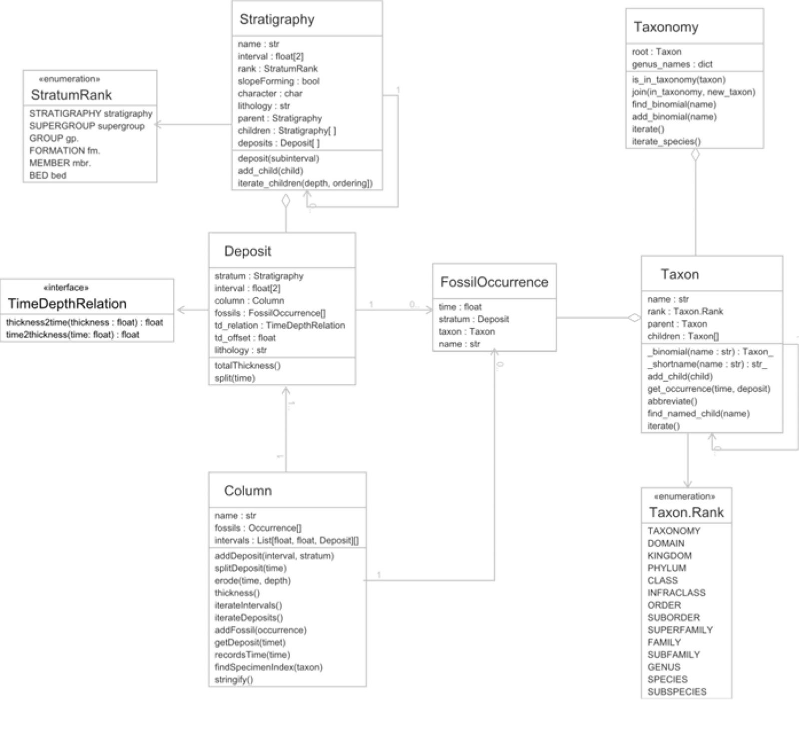
Fig. 1. UML Class diagram of the stratigraphy package structure and methods.
The simulation is given an initial overall seed which is used to ensure repeatability of any particular run in the random simulation. If no starting seed is given, then one is chosen randomly. The seed used is retained and reported to the user at the start of the simulation run. The initial master seed is used to deterministically spawn additional seeds which are used to initialize independent bit stream generators for every process which requires a random output. Separately initialized bit generators ensure that the outputs of each are independent of each other, and random outputs are stable following code changes, except of course for the portion of code that is modified. When multiple simulations are set up and run to produce a statistical distribution, the seeds for each simulation run are likewise generated from a single master seed and fed to each simulation instance for initialization. This method allows consistent seed generation and propagation for parallel processing.
Random bit generators are used in the simulation to determine the deposition time of fossil occurrences as well as setting the variance on the distribution of number of occurrences (when applicable) and applying gloss to columns and taxa.
Fossil Relationships Graph Analysis
In the case of the biostratigraphy simulation, all of the taxa in the fossil record are represented in a graph by vertices, with edges representing whenever occurrences of two taxa can be stratigraphically linked to each other (that is, by being found in the same column). This is equivalent to the biostratigraphic graph G* of the UAM. Definitions of graph theory concepts can be found in the appendix.
Edges summarize all of the relationship combinations that are found between occurrences of fossil taxa throughout the entire fossil record. There are two types of relationships between fossil taxa that are represented in the graph. The relationship of first importance is whether or not a taxon is always found stratigraphically above another in all of the columns where both can be found. This edge is directed from the higher taxon to the lower taxon. These edges will be collectively referred to as the “Always Above” edge set. The most common relationship is an undirected edge representing that the two taxa are found together with both taxa being above and below the other in various columns (tables 1 and 2).
The properties of directed acyclic graphs (DAGs) are essential in being able to perform the path finding algorithms described below. As it will be shown in the next section, biostratigraphy also relies implicitly on a subgraph of fossil relations being a DAG.
| Column 1 | Column 2 | |
|---|---|---|
| Stratum X | A. exemplum | A. exemplum |
| Stratum Y | B. aliae | B. aliae |
Table. 1. Example fossil record where A. exemplum is always above B. aliae (A. exemplum → B. aliae).
| Column 1 | Column 2 | |
|---|---|---|
| Stratum X | A. exemplum | B. aliae |
| Stratum Y | B. aliae | A. exemplum |
Table 2. Example fossil record where A. exemplum and B. aliae are found both above and below each other (A. exemplum ↔ B. aliae).
Criteria for valid biostratigraphic fossil set
To produce a valid fossil ordering, a chain of fossil taxa which are consistently found above each other is necessary. This “aboveness” (superposition) defines an asymmetric directionality to the fossil relationships which forms a path of increasing length over geologic time. In general, this directed path is a subgraph of all fossil taxa relations. In this model, each of the identified taxa are treated as index fossils, where the time interval over which these fossils may be found is defined as the period for which other fossils and events are indexed. Because of the directed relationships, these index intervals are all disjoint from each other. Meaning that no more than one index fossil taxon can be found in any one interval. Formally described, this simulation is setup to consider interval biozones based on first appearance datums (FADs), though more complicated modern biostratigraphic concepts, such as assemblage biozones or unitary associations, could be considered as “pseudo-taxa” and would produce equivalent results.
To be valid, the index taxa must be consistently transitively related by superposition with all other index taxa. That is to say, if any taxon A is always above taxon B which is immediately before it in the time scale, then it should always be above any taxa C which B is always above, whenever they are found together. The graph implication of this is that there can be no cycles (loops) in the index fossil induced subgraph. This also ensures that the chosen index fossil set has a consistent total ordering.
The selection of an index fossil set introduces a strict partial ordering on the entire Fossil Taxa Relations graph, given that the relationships are both transitive and asymmetric (Flaška et al. 2007). The more taxa are represented in the index fossil subset, the more complete is the partial ordering. This comes both from having smaller divisions over the entire span of geologic time, yielding more finetuned time determinations, but it also increases the number of taxa which are connected to the timescale.
We can now mathematically describe the process of biostratigraphy as finding the longest directed acyclic induced path in the Fossil Taxa Relations graph, where each period in the time scale is defined as the interval over which the relevant index fossil is found. Such a formulation may sound alien to the traditional methods that were established at the beginning of geology, but it is closely in line with the formalisms of modern biostratigraphers, particularly the UAM.
Path Finding Algorithm
The longest path finding algorithm begins by creating an edge-induced subgraph of the in the Fossil Taxa Relations graph with the Always Above edge set which includes no bidirectional relationships between Taxa. This subgraph is directed, satisfying the first criteria of a DAG.
To find the longest path, the subgraph additionally needs to be acyclic. This is achieved on the subgraph by computing the feedback arc set of the graph, which is the set of edges (arcs) whose removal will ensure the graph is DAG. The algorithm used to find a feedback arc set is that of Eades, Lin, and Smyth (1993). Because fossil relationships cannot be simply ignored to generate a valid biostratigraphy, the edges are removed by eliminating associated vertices one-by-one in the feedback arc set edge-induced subgraph, that is, fossil taxa are individually removed from consideration as index fossils.
Because the feedback arc set specifies which edges should be removed, there are multiple permutations of vertices to remove to break the necessary relationships. This algorithm uses the first solution found with the minimal number of vertices removed. This is guaranteed to produce an optimal solution to the minimal vertex cover of the feedback arc subgraph but does not guarantee optimality in the maximal path length in the final solution.
For most algorithm steps, the runtimes of the above algorithms are linear in the number of vertices plus the number of edges in the graph. However, finding the minimal number of vertices to remove to form a DAG is a variant of the Minimal Vertex Cover problem, which is NP-hard and runs in exponential time with the size of the feedback arc set induced subgraph. This is the main runtime bottleneck in the simulation, particularly for larger graphs with large feedback arc sets. It was found that a quick-running greedy algorithm solution removed too many taxa, so the resulting index fossil set was severely reduced, and in many cases could not be found due to the entire graph becoming disconnected. The above steps ensure that the resulting subgraph is acyclic, satisfying both criteria to be a DAG.
Once a directed acyclic subgraph is found, then a topological ordering on the resulting subgraph was computed. A topological ordering is an ordered listing of all of the vertices in a graph where each vertex is listed before all of its successor vertices as defined by the directional relationships. Topological orderings are guaranteed to exist if the subgraph is a DAG, and are not unique. The topological sorting is performed with a depth-first search.
The next step is to step through each of the vertices in order, marking down the longest distance to arrive at that node as the maximal distance to any of its successors plus one, with the first vertex being at distance 0. The longest path through the subgraph is then the maximal distance value marked for any vertex in the entire set. The vertex with the highest distance value is chosen for the candidate path and its predecessors evaluated, choosing the predecessor with the highest distance value, until the starting vertex is reached, which yields a candidate longest path.
The candidate longest path was constructed with only a subset of the potential relationships, and it is possible for a bidirectional relationship in the full graph that we ignored in the first step to cause it to by cyclic, so the found candidate longest path is used to create a subgraph of the full, mixed-directionality Fossil Taxa Relations graph. The resulting subgraph is used to check to see if the candidate is still valid (DAG) with all relationships. The above algorithm is iterated with additional candidate subgraphs (removing additional taxa from consideration) until one is found which is valid for the entire graph.
As a fallback, if a solution can’t be found with the Always Above graph, then the algorithm is repeated with the full Fossil Taxa Relations graph. This fallback takes a significantly longer amount of time to run.
Biostratigraphy Algorithms
Timescale construction
The index fossil list found via graph analysis is the basis for constructing a valid simulated time scale with one period per index taxon. One additional period is added at the beginning to account for time before the first appearance of the first index fossil. Additional information is gathered by looking at the relative positioning of the index fossils in each column. A proxy for time is found by counting the maximal number of formations which each period in the timescale covers. This is found in three steps:
- Find the lowest occurrence of the youngest index fossil to determine how many rock formations are found above the latest index fossil first occurrence.
- Find columns containing boundaries between all adjacent index fossils to determine the maximum number of rock formations between the index fossil occurrences.
- Find the highest occurrence of the oldest index fossil to determine how many rock formations are found below the first index fossil occurrence.
All of the columns which provided the key information during the search are collected into a type sections list.
Column Painting
Once the maximal number of formations that each time scale period covers is determined, then there is sufficient information to estimate the time scale period applied to each deposit in columns which contain at least one index fossil. I term this process “painting.” Painting the columns supports the ability to assign date ranges to non-index fossils within the constructed time scale.
Not every deposit in every column has an index fossil to directly “date” the deposit. This leaves a time ambiguity based on the physical evidence, which in reality would be filled in by other methods. For the purposes of the simulation, there is enough information to make an estimated guess. When there are two adjacent index fossils, then it is reasonable to assume that the formations below the first appearance of the second belong to the first’s period. Similarly, formations below the first appearance of an index fossil are likely to belong to the immediately preceding period. These guesses are not guarantees, since there is no way to truly know if the first appearance of a taxon in a particular column represents the absolute first appearance of that taxon. Also, when there is a jump of greater than one period indicated by the index fossils, then there are multiple possible appropriate periods between. The model deals with this ambiguity by assuming that number of known formations spanned by a timescale period is allowed to “paint” up to the same number of formations in any particular column. Once the maximal number of formations with paint applied has been reached, then the “paint” advances to the next period. In the case when two index fossils are found in the same deposit, then the backwards paint applied is prior to the older index fossil, and the forward paint applied corresponds to the younger fossil.
The painting algorithm also provides important updates to the timescale in the form of detecting required implied expansions to the timescale periods. The cases which these cover involve finding maximal formations between occurrences of the same index fossil, or between non-adjacent index fossils that are not considered by the timescale construction algorithm. Each extension detected causes the column which necessitated the adjustment to be added to the type sections list. This algorithm can also detect an index fossil range extension if new occurrences of index fossils have been added since the graph analysis. Because of this modification function, this process is repeated twice, one to detect time scale expansions, then once more to actually apply the paint to the columns.
The painting algorithm examines each column with at least one index fossil, proceeding as follows:
- Find the first transition represented by the lowest index fossil.
- Paint deposits backwards with the previous time scale period to the bottom of the column.
- If this would involve painting beyond the end of the time scale, then the pre-oldest taxon period is extended as necessary
- Start from the first transition again and paint deposits forwards.
- For each deposit, check the fossil content for index fossils.
- Advance the paint period to correspond with the new index fossil. If this requires moving the period backwards (earlier), then the prior period is extended.
Biozones and Range Extensions
Once all of the columns which have an index fossil have been painted and the timescale has been established, the method to find faunal ranges for non-index taxa is equivalent to Shaw’s Graphical Correlation method. The painted columns are used to assign deposition ages to all of the non-index fossil occurrences which occur in one of the painted columns based on the paint of the deposit in that column. These are aggregated per fossil taxon over the entire column set to determine first and last appearances of all fossil taxa.
Following this step, columns which do not contain any index fossils are examined for fossil taxa range extensions. Given that these columns do not have any index fossils, they are not subject to direct age control. Their non-index fossil content however does provide a form of secondary age control. Whenever this leads to an inconsistency between the first and last appearances established by primary age control, this results in an age extension for one or more of the fossil taxa. The simulation detects required age extensions by comparing if the last known appearance of the higher occurrence is older than the first known appearance of the lower occurrence. There are multiple ways that the range extension could be adjudicated, which the simulation does not attempt to decide. It simply notes the extension and adds the column to the type sections list.
Fossil age ranges are estimated by using the number of units in chronostratigraphic periods as a time proxy, with ages assumed to be at the start of the relevant period.
Mathematical Proof of Guaranteed Biostratigraphic Solution
The graph theory definitions required to prove that there is a biostratigraphic method that will guarantee a result which can be interpreted as a set of valid intervals can be found in the appendix.
Lemma 1. Pairs of fossil taxa with the “Above and Below” relationship implies that their true (hidden) deposition intervals overlap.
Proof. Any fossil occurrence is found in its taxon deposition interval, and the time between the deposition of two occurrences is also on the interval.
When the “above and below” relationship can be established in a single column, then an occurrence of one of the taxa must be between two occurrences of the other, so the two intervals overlap.
Otherwise, for a pair of fossil taxa A, B to have the “above and below relationship,” there exist two columns with occurrences of both A and B of which one has A above B and the other with B above A.
Without loss of generality, consider the oldest occurrence of taxon A to be in column 1, with the youngest in column 2. There are two cases: the occurrence of taxa B in column 1 must be either above or below the oldest occurrence of taxon A. Consequently, in column 2, the occurrence of B must have the opposite relationship with the youngest occurrence of A.
Case 1
In the case of B in column 1 being below the oldest occurrence of A, then that occurrence is also older than the youngest occurrence, and the occurrence of B in column 2 is younger than both occurrences of A, so the interval of B completely covers the interval between the two occurrences of A, so the two intervals overlap.
Case 2
In the case where B in column 1 is above the oldest occurrence of A, the deposition age of the occurrence of B is only constrained from below, and could possibly be younger than both occurrences of A. When the occurrence of B in column 1 is deposited between the two occurrences of A, then the fact that the intervals overlap is clear.
The final subcase to check is when the occurrence of B in column 2 is younger than the youngest occurrence of A. In this final subcase, the occurrence of B in column 2 then is younger than both the youngest occurrence of A and the occurrence of B in column 1, so the youngest occurrence of A is contained in the interval of B.
Theorem 1. The biostratigraphic method will always produce fossil depositions ranges as valid intervals that in general will not match the true (hidden) intervals.
Proof.
- The full (hidden) graph of fossil time relations can be constructed as an interval graph.
Therefore, it is AT-free and chordal. - The “Above and Below” edge induced subgraph of the fossil record is a subgraph of the hidden full interval graph from lemma 1 above.
Therefore, there is at least one solution for completing the fossil record graph which is a valid interval graph. - Solutions are not unique.
Intervals can be shrunk through incomplete knowledge. Interval intersections will be lost, but the resulting interval graph is always a subgraph of the full graph. - Removal of edges from the full fossil relations graph to arrive at the presently known fossil record will never create an asteroidal triple, since that is based on path existence and removal of an edge does not cause the creation of a path that did not exist before.
Therefore, the fossil record is AT-free. - The fossil record may be missing necessary chords for the graph to be chordal, so a biostratigraphic solution will be constructed by adding edges until the graph is chordal.
- When adding chords the possibility exists that a new asteroidal triple might be created, so we apply a constraint that all added chords in the solution do not create asteroidal triples (ATs).
Adhering to this constraint is always possible since it is guaranteed that at least one such solution exists from step 2 above. - Therefore, it is always possible to construct an interval graph from the available fossil record, and given the non-uniqueness of solutions, the solution is not guaranteed to correspond to the true (hidden) solution.
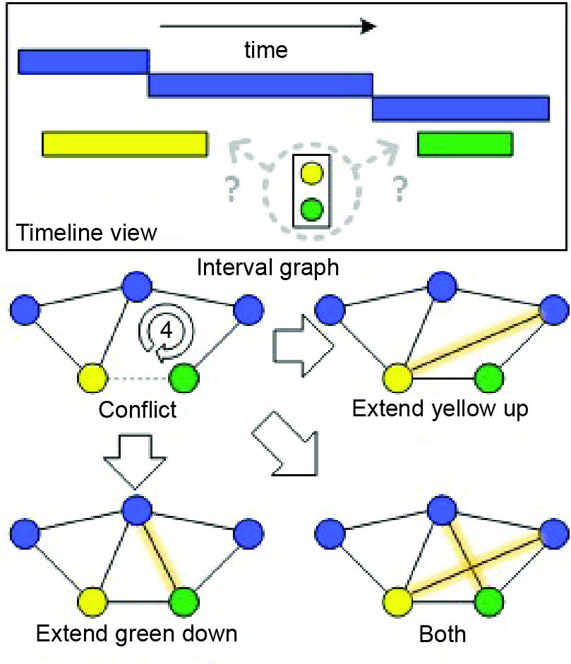
Fig. 2. Timeline with interpreted deposition intervals for a set of taxa, and the discovery of an out-of-order pairing between the yellow and green taxa. Blue taxa are index intervals. Bottom shows the interval graph representation of the conflict and three possible resolutions.
Interval graphs are non-unique to reversal of the timescale. Superposition relationships add additional context that is not in a traditional interval graph, but which must be accounted for to construct a time scale. Some of this information can be accounted for by assuming that all of the index intervals have an infinitesimal overlap with their immediate neighbors. In the full hidden interval graph, the true “always above” relationships form a directional compliment to the interval graph. So, combining both the interval graph and its compliment result in a perfect graph where every interval has a relationship with every other interval, either overlapping or non-overlapping with an ordering in time.
Whenever there is a cycle of four or more vertices in the fossil record, then a chord must be added to create a valid interval graph. This corresponds to making a range extension. One possible chord choice corresponds to extending the last occurrence of one taxon, while the other chord choice corresponds to lowering the first occurrence of the other taxon (Fig. 2).
Conclusion
The automated biostratigraphic algorithms outlined in this paper are consistent with the modern and historical practices in biostratigraphy so provide a suitable platform for testing the effectiveness of biostratigraphy when the core assumption of faunal succession does not or only partially holds true. The ability to directly compare differing Flood burial scenarios with respect to their expected ordering and the effect of assuming faunal succession is a novel contribution to Flood geology. It was also proved mathematically that there are multiple potential orderings that are valid for a given biostratigraphic interpretation. The conclusion that these multiple orderings must be mutually contradictory was neither proven nor eliminated as a possibility.
References
Agterberg, F. P., and F. M. Gradstein. 1999. “The RASC Method for Ranking and Scaling of Biostratigraphic Events.” Earth-Science Reviews 46, nos. 1–4 (May): 1–25.
Eades, Peter, Xuemin Lin, and W. F. Smyth. 1993. “A Fast and Effective Heuristic for the Feedback Arc Set Problem.” Information Processing Letters 47, no. 6 (18 October): 319–323.
Edwards, Lucy E. 1984. “Insights on Why Graphic Correlation (Shaw’s Method) Works.” Journal of Geology 92, no. 5 (September): 583–597.
Edwards, Lucy E. 1995. “Graphic Correlation: Some Guidelines on Theory and Practice and How They Relate to Reality.” In Graphic Correlation. Vol. 53. Edited by K. O. Mann, H. R Lane, and P. A. Scholle, 45–50. Tulsa, Oklahoma: SEPM Society for Sedimentary Geology.
Flaška, V., J. Ježek, T. Kepka, and J. Kortelainen. 2007. “Transitive Closures of Binary Relations. I.” Acta Universitatis Carolinae Mathematica et Physica 48, no. 1: 55–69.
Galster, Federico, Jean Guex, and Oyvind Hammer. 2010. “Neogene Biochronology of Antarctic Diatoms: A Comparison between Two Quantitative Approaches, CONOP and UAgraph.” Palaeogeography, Palaeoclimatology, Palaeoecology 285, nos. 3–4 (15 January): 237–247.
Guex, Jean. 1991. Biochronological Correlations. Heidelberg, Germany: Springer.
Guex, Jean. 2011. “Some Recent ‘Refinements’ of the Unitary Association Method: A Short Discussion.” Lethaia 44, no. 3 (8 July): 247–249.
Guex, Jean, and Eric. Davaud. 1984. “Unitary Associations Method: Use of Graph Theory and Computer Algorithm.” Computers and Geosciences 10, no. 1: 69–96.
Kemple, William G., Peter M. Sadler, and David J. Strauss. 1995. “Extending Graphic Correlation to Many Dimensions: Stratigraphic Correlation as Constrained Optimization.” In Graphic Correlation. Vol. 53. Edited by K. O. Mann, H. R Lane, and P. A. Scholle, 65–82. Vol 53. Tulsa, Oklahoma: SEPM Society for Sedimentary Geology.
MacLeod, Norman, and Peter M. Sadler. 1995. “Estimating the Line of Correlation.” In Graphic Correlation. Vol. 53. Edited by K. O. Mann, H. R Lane, and P. A. Scholle, 51–64. Vol 53. Tulsa, Oklahoma: SEPM Society for Sedimentary Geology.
Monnet, Claude, Arnaud Brayard, and Hugo F. R. Bucher. 2015. Ammonoids and Quantitative Biochronology—A Unitary Association Perspective. In Topics in Geobiology 44. Edited by N. H. Landman, E. A. Erwin, N. J. Mutti, and G. B. Vai: 277–298. Heidelberg, Germany: Springer.
O’Neill, Melissa E. 2014. “PCG: A Family of Simple Fast Space-Efficient Statistically Good Algorithms for Random Number Generation.” Technical Report HMCCS-2014-0905 (September). Claremont, California: Harvey Mudd College.
Puolamäki, K., Mikael Fortelius, and Heikki Mannila. 2006. “Seriation in Paleontological Data Using Markov Chain Monte Carlo Methods.” PLoS Computational Biology 2, no. 2 (February 10): e6.
Sadler, Peter M. and Roger A. Cooper. 2008. “Best-Fit Intervals and Consensus Sequences.” In High-Resolution Approaches in Stratigraphic Paleontology. Topics in Geobiology 21. Edited by Peter J. Harries: 50–94. Heidelberg, Germany: Springer.
Shaw, Alan B. 1964. Time in Stratigraphy. Vol. 1. New York, New York: McGraw-Hill.
Zhang, Tao, and Roy E. Plotnick. 2006. “Graphic Biostratigraphic Correlation Using Genetic Algorithms.” Mathematical Geology 38 (October): 781–800.
Appendix: Graph Theory Definitions
A graph is a set of vertices and a set of edges which connect pairs of vertices together.
Edges which connect two vertices may be directed or undirected. With directed edges, there is a predecessor and successor relationship between the connected vertices. With undirected edges, the endpoints are interchangeable, or the relationship is bidirectional. Edges are sometimes called arcs.
A subgraph is a graph whose vertices and edges are subsets of the vertices and edges of another graph. When a subgraph contains all of the edges between the subset of vertices in the original graph, then it is called a vertex-induced subgraph (or most commonly just induced subgraph). When a subgraph contains all vertices specified by a subset of edges, then it is called an edge-induced subgraph.
A path is a sequence of edges which joins a sequence of distinct vertices. When the edges are directed, then it is known as a directed path. An induced path is an induced subgraph that is also a path.
A directed acyclic graph (DAG) is a graph with directed edges which includes no cycles (loops). This means that there is no way to arrive at any particular vertex twice by following the edges without backtracking.
A chordal graph is one in which all induced paths which include cycles of 4 or more nodes have a chord, which is an edge that is not part of the cycle, but which connects two nodes.
Three vertices of a graph form an asteroidal triple (AT) when there exists a path between every pairing which connects the two without including any vertices from the neighborhood of the third. A graph which contains no asteroidal triples is said to be AT-free.
An interval graph is a graph where intervals are represented as vertices and edges represent when two intervals overlap. A graph is an interval graph if it is 1) chordal and 2) AT-free.
A compliment graph is a graph which contains the same vertices as another graph, but has an edge between every node pair that did not have an edge in the original graph, and has no edge where there was one. The union of a graph and its complement results in a perfect graph where all vertices have edges to all other vertices.