Size of Galaxies in JWST Data and Cosmology— Reply to Lisle

Introduction

The Friedmann-Lemaitre-Robertson-Walker (FLRW) model of the expansion of space provides the dominant framework for modern cosmology. When combined with a set of parameters derived from observations of the cosmic microwave background (CMB), galaxy redshift surveys, and more, this model is often called the standard model of cosmology (Planck Collaboration 2020; Scott 2018). With Prof. Geraint Lewis, I have given a popular-level account of the strengths and weaknesses of the model in Barnes and Lewis (2020)

The model predicts the relationship between the physical size of a distant object and its apparent (angular) size. The angular diameter distance (D_A) is defined so that, for an object whose proper transverse size is L, its measured angular extent θ is,

The calculation of D_A takes into account the expansion history of the universe; more details can be found in Hartle (2021), Hogg (1999), and Liddle (2003).

For a given galaxy in the night sky, θ is directly observed, D_A is derived from a model of spacetime, and L is inferred from these two quantities. If we had a population of objects of known physical size throughout the universe (standard rulers), we would be able to use them to test the cosmological model and constrain its free parameters. However, the universe is unfortunately not filled with luminous rigid rulers of known sizes. What we have are galaxies: gravitationally-bound collections of stars, gas, and (in the standard model) dark matter. Thus, to see whether the observed distribution of galaxy angular sizes is consistent with a given model of spacetime, we need to be able to derive predictions for the physical sizes of galaxies from the standard cosmological model.

Recently, Lisle (2024) has argued that the distribution of galaxy angular sizes is inconsistent with the standard model of cosmology. Here, we will compare his model for the physical sizes of galaxies with one based in modern galaxy formation theory. We will outline the models in the Introduction. The next section (Modelling the Physical Sizes of Galaxies) will compare the results of the models. The third section (Model Predictions and Comparison with Data) will outline our conclusions.

Modelling the Physical Sizes of Galaxies

Self-gravitating systems are complicated. For a system of two gravitating bodies, we can exactly solve Newton’s law of gravity on paper. For three bodies, we can’t. Einstein’s theory of gravity (General Relativity) adds another layer of difficulties. For a galaxy, consisting of hundreds of billions of stars, clouds of gas, and dark matter, we understand their behaviour using a range of statistical analytical methods, numerical calculations, and semi-analytical models that combine aspects of each. The interested reader should consult the textbook of Mo, van den Bosch, and White (2010).

Here, we will use a semi-analytic model to predict the size distribution of galaxies in the standard model. The Theoretical Astrophysical Observatory (TAO)1 provides free, publicly-available online access to the Semi-Analytic Galaxy Evolution (SAGE) model, presented in Croton et al. (2016). Here is a brief introduction to physical processes modelled in SAGE.

1. An N-body (gravity only) supercomputer simulation of dark matter provides the merging hierarchy of structure in which galaxies form. These simulations begin with an almost uniform distribution of matter, and calculate the gravitational pull of matter-on-matter in an expanding space to follow the growth of structure. TAO provides six N-body simulations; here we use a simulation called “MultiDark”2 (Klypin et al. 2016), which uses 57 billion simulated particles to follow a region of the universe that expands to be 1,475 Mpc (4.8 billion light years) across today.

2. Regions of matter that collapse to be gravitationally bound are referred to as haloes. These are identified in the simulation using the Bound Density Maxima (BDM) halofinder (Klypin and Holtzman 1997; Riebe et al. 2013).

3. Haloes that merge will form a new, larger halo. The smaller halo in the merger will have some of its gas stripped by ram pressure from the larger halo. The timescale for the merger is calculated from considerations of dynamical friction.

4. Gas that falls into a halo is subject to cooling via radiation, and heating from Active Galactic Nuclei (AGN). Sufficiently strong feedback from AGN and supernovae can eject gas back into the circum- and inter-galactic medium. Haloes contain hot gas in their haloes, whose accretion rate into the halo is determined by the gas’s cooling rate.

5. Within a galaxy, the ecosystem of mass is followed, as baryons cycle through interstellar gas, stars, galactic winds, and black holes. In particular, cold gas will form a rotationally supported disk of gas and stars. The disk radius (r_disk) is given by,

   $$r_{disk}=\frac{3}{\sqrt{2}}\lambda R_{vir},$$ (2)

   where λ is the spin parameter of the dark matter halo, and R_vir is the virial radius of the dark matter halo, which are both calculated in the N-body simulation.

6. Gravitationally bound disks can form instabilities. Under these conditions, the gas in the disk is unstable to collapse into bound, star-forming clouds, as described by the Kennicutt-Schmidt relation. The unstable gas will also feed a central supermassive black hole. Accretion of matter onto the black hole powers an AGN.

7. The free parameters of the model were constrained to reproduce the distribution of galaxy stellar masses today (redshift z = 0). The model successfully reproduces the average cosmic star formation rate as a function of redshift (out to z = 5), the baryonic Tully-Fisher relation at z = 0, and the stellar mass-gas metallicity relationship at z = 0.

8. For our purposes, a simulation of a galaxy survey was run on TAO, for a region of the sky that is 2° × 2° in angular size, and extends from z = 1 to z = 12. From TAO, the following quantities were extracted for each galaxy: total stellar mass, disk scale radius, halo total mass, halo virial radius, and redshift. The relevant cosmological parameters are those for the MultiDark simulation.3 TAO provides a simple, publicly available web interface for generating a simulation, which is available for the user to download after a few hours.

We can also list the postulates of the Lisle (2024) model for the physical sizes of galaxies.

1. Galaxies have the same average size (4.5 kpc) everywhere and at all times.

Model Predictions and Comparison with Data

Using the population of galaxies predicted by SAGE, calculated in TAO, we calculate the average angular diameter of galaxies in redshift bins. The results are shown in fig. 1.

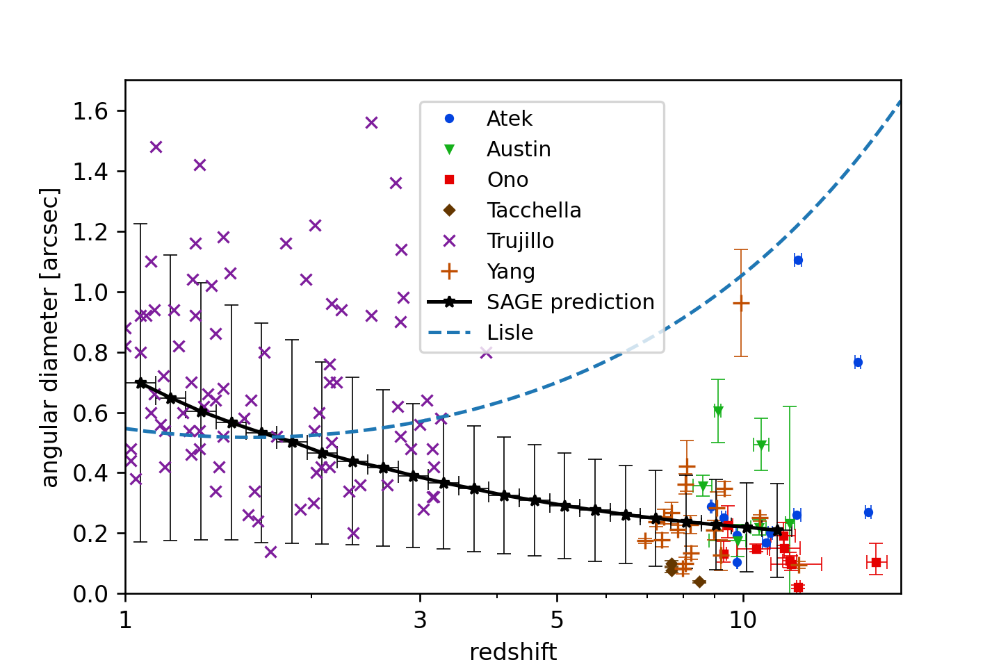
Fig. 1. Angular diameters of galaxies, as a function of redshift. The six coloured markers show redshift and angular diameters from (Atek et al. 2023; Austin et al. 2023; Ono et al. 2023; Tacchella et al. 2023; Trujillo et al. 2004; Yang et al. 2022). These are the same data sources as those used by Lisle (2024). Where available, we have included 1 sigma error bars around data points. Specifically, the angular diameter is twice the “effective radius” of the source, calculated by fitting a Sérsic profile. The solid black line shows the mean angular diameter in arcsec, in the redshift bins shown, for simulated galaxies in the SAGE semi-analytic model. The vertical bars show one standard deviation in the properties of the disks at each redshift. Note well: these bars represent the width of a distribution; they are not the error in the mean. The dashed blue line shows the “standard model” prediction of Lisle (2024).

Following Lisle (2024), we show observations of galaxy angular sizes at various redshifts for six surveys: Atek et al. 2023; Austin et al. 2023; Ono et al. 2023; Tacchella et al. 2023; Trujillo et al. 2004; Yang et al. 2022). Where available, we have included 1 sigma error bars around data points. Specifically, the angular diameter is twice the “effective radius” of the source, calculated by fitting a Sérsic profile.

In fig. 1, the solid black line shows the mean angular diameter in arcsec, in the redshift bins shown, for simulated galaxies in the SAGE semi-analytic model. The vertical bars show one standard deviation in the properties of the disks at each redshift. Note well: these bars represent the width of the distribution; they are not the error in the mean. The dashed blue line shows the “standard model” prediction of Lisle (2024). Two conclusions are immediately apparent. Firstly, the prediction from the standard model of cosmology is consistent with the data, including the new data above z = 7. If anything, the model may fail to capture a population of large galaxies around z ~ 2 − 3. However, there are a number of physical effects that the model does not capture. We have not attempted to model the effects of galaxy survey selection criteria (including photometric dropouts), the effect of dust absorption, and processes relevant to galactic sizes such as spiral arm, bar and bulge formation, star scattering, vertical heating, radial migration, minor mergers, major mergers, and more. Nevertheless, the model captures the most important effect: the merging and growing of haloes, and the corresponding increase in their galaxy sizes with time. By modelling the evolution of this hierarchical structure, the SAGE model shows an adequate consistency with observations. Note well: the SAGE model was published in 2016, so its parameters were not tweaked to reproduce the observations of JWST, which launched in 2021.

Secondly, the “standard model” prediction of Lisle (2024) bears no resemblance to the actual predictions of the standard model. The assumption that average galaxy sizes are constant with redshift is inadequate. No method of calculating the growth of structure in the standard model predicts this. The increase in masses and physical sizes of haloes and their associated galaxies with time is a firm prediction of analytic, N-body and hydrodynamical simulations of galaxy formation. These models are no secret. As well as the TAO semi-analytic models described here, there are publicly available hydrodynamic simulations of galaxy formation.4 There are also publicly available code packages that calculate the analytic properties of haloes using the extended Press-Schecter formalism.5 In light of these resources, the “standard model” prediction of Lisle (2024) is both inadequate and inexcusable. It is a straw man.

We conclude that the observed sizes of galaxies are consistent with the standard model of cosmology. This point should not be overstated: the sizes are some evidence in favour of the model, but far from decisive. The prediction of galaxy sizes involves a variety of messy astrophysical processes, most of which we can only approximate. Galaxies aren’t rigid. Nevertheless, the charge of inconsistency against the standard model clearly fails.

Conclusions

Given the inadequacy of the “standard model” prediction of Lisle (2024), his attempts to perform the Tolman Test should be disregarded. This is a famously difficult observational test, because galaxies are not “standard candles,” of uniform and predictable luminosity. Allan Sandage, one of the greatest astronomers of the twentieth century (and a Christian), spent decades attempting to perform this test. Writing in 2010, in one of a series of five papers that he published on the Tolman Test, he comments:

the Tolman test . . . has not been quite as easily done as I set out . . . in 1974. It has required many developments not yet made at the time. However, the test seems to have been successful. The Tolman prediction is verified. The expansion would seem to be real. (Sandage 2010)

Lisle (2024) has not even attempted to wrestle with the messy astrophysics required to complete the test—stellar evolution and K-corrections, amongst other things. Thus, no inconsistency can be demonstrated.

It is incorrect for Lisle (2024) to argue that his results “suggest that the redshifts of galaxies are entirely the result of a relativistic Doppler effect in non-expanding space.” As explained in Peacock (1999, 87), redshifts in all “expanding space” models (FLRW) can be calculated as an accumulation of small Doppler shifts, caused as light travels between neighbouring comoving observers. In other words, the difference between the “expanding space” picture and the “Doppler” picture is a mere change in perspective, a coordinate transformation. General Relativity is founded on coordinate-independence.

In that case, what is the “Doppler Model” of Lisle (2024)? It’s another Big Bang model. This can be shown as follows. Equation (10) from Lisle (2024) shows that the “Doppler distance” is equivalent to the angular diameter distance (D_A). In a flat FLRW model:

This expression can be set to be equal to equation (9) from Lisle (2024), from which can be derived the redshift dependence of the RW Hubble parameter $H(z)$. Given that $H(z)=\acute{\alpha }/\alpha$ and $\alpha =1/(1+z)$, this expression can be inverted to give $\alpha (t)$ for the “Doppler Model.” (Unfortunately, the equations cannot be analytically inverted, so we cannot provide a simple formula. However, the solution exists and would not be difficult to calculate numerically.) In this model, equations (9) and (10) of Lisle (2024) hold, and a version of the Hubble law that relates the angular diameter distance and the “velocity” as derived from the redshift via the special relativistic relation (Lisle, 2024, eqn. 8) also holds.

Thus, the “Doppler Model” of Lisle (2024) is physically indistinguishable from an expanding space model. It is a mere redescription. The only difference is a change of coordinates, which aren’t physically observable. In both the Doppler Model and the standard model, the finite speed of light will make the universe appear to be billions of years old, so supporting the first while criticising the second does nothing to solve the Starlight and Time problem. Lisle proposes to solve this with the Anisotropic synchrony convention, which implies that we see galaxies as they are now, regardless of how far away they are. This gives the model enough freedom that any observed population of galaxies is consistent with a young universe. In that case, one might as well attach the convention to the Big Bang model and be done with it.

References

Atek, Hakim, Marko Shuntov, Lucas J. Furtak, John Richard, Jean-Paul Kneib, Guillaume Mahler, Adi Zitrin et al. 2023. “Revealing Galaxy Candidates out to z ~ 16 with JWST Observations of the Lensing Cluster SMACS0723.” Monthly Notices of the Royal Astronomical Society 519, no. 1 (February): 1201

Austin, Duncan, Nathan Adams, Christopher J. Conselice, Thomas Harvey, Katherine Ormerod, James Trussler, Qiong Li, Leonardo Ferreira, Pratika Dayal, and Ignas Juodžbalis. 2023. “A Large Population of Faint 8 <z <16 Galaxies Found in the First JWST NIRCam Observations of the NGDEEP Survey.” The Astrophysical Journal, 952, no. L7. DOI 10.3847/2041-8213/ace18d.

Barnes, Luke A., and Geraint F. Lewis. 2020. The Cosmic Revolutionary’s Handbook (Or: How to Beat the Big Bang). Cambridge, UK: Cambridge University Press.

Croton, Darren J., Adam R. H. Stevens, Chiara Tonini, Thibault Garel, Maksym Bernyk, Antonio Bibiano, Luke Hodkinson, Simon J. Mutch, Gregory B. Poole, and Genevieve M. Shattow. 2016. “Semi-Analytic Galaxy Evolution (SAGE): Model Calibration and Basic Results.” The Astrophysical Journal Supplement Series, 222, no. 22 (February 18). DOI 10.3847/0067-0049/222/2/22.

Hartle, James B. 2021. Gravity: An Introduction to Einstein’s General Relativity. Boston, Massachusetts: Addison Wesley.

Hogg, David W. 1999. “Distance Measures in Cosmology.” arXiv e-prints,astro- ph/9905116.

Klypin, Anatoly, and Jon Holtzman. 1997. “Particle-Mesh Code for Cosmological Simulations.” arXiv e-prints,astro-ph/9712217.

Klypin, Anatoly, Gustavo Yepes, Stefan Gottlöber, Francisco Prada, and Steffen Heß. 2016. “MultiDark Simulations: The Story of Dark Matter Halo Concentrations and Density Profiles.” Monthly Notices of the Royal Astronomical Society 457, no. 2 (1 April): 1137–1144.

Liddle, Andrew. 2003. An Introduction to Modern Cosmology. 2nd ed. Hoboken, New Jersey: John Wiley and Sons.

Lisle, Jason. 2024. “Sizes of Galaxies in JWST Data Suggest New Cosmology.” Answers Research Journal 17 (July 24): 445–457. https://answersresearchjournal.org/cosmology/jwst-data-suggest-new-cosmology/.

Mo, Houjun, Frank van den Bosch, and Simon White. 2010. Galaxy Formation and Evolution. Cambridge, UK: Cambridge University Press.

Ono, Yoshiaki, Yuichi Harikane, Masami Ouchi, Hidenobu Yajima, Makito Abe, Yuki Isobe, Takatoshi Shibuya, John H. Wise, Yechi Zhang, Kimihiko Nakajima, and Hiroya Umeda. 2023. “Morphologies of Galaxies at z >9 Uncovered by JWST/NIRCam Imaging: Cosmic Size Evolution and an Identification of an Extremely Compact Bright Galaxy at z~12.” The Astrophysical Journal 951, no. 1 (July 1): 72. DOI 10.3847/1538-4357/acd44a.

Planck Collaboration, N. Aghanim, Y. Akrami, M. Ashdown, J. Aumont, C. Baccigalupi, M Ballardini, et al. 2020. “Planck 2018 results. VI. Cosmological Parameters.” Astronomy and Astrophysics 641 (September): A6. https://doi.org/10.1051/0004-6361/201833910.

Riebe, K., A. M. Partl, H. Enke, J. Forero-Romero, S. Gottlöber, A. Klypin, G. Lemson, F. Prada, J. R. Primack, M. Steinmetz, and V. Turchaninov. 2013. “The MultiDark Database: Release of the Bolshoi and MultiDark Cosmological Simulations.” Astronomische Nachrichten 334, no. 7 (August): 691–708.

Sandage, Allan. 2010. “The Tolman Surface Brightness Test for the Reality of the Expansion. V. Provenance of the Test and a New Representation of the Data for Three Remote Hubble Space Telescope Galaxy Clusters.” The Astronomical Journal 139 (February): 728.

Scott, Douglas. 2018. “The Standard Model of Cosmology: A Skeptic’s Guide.” arXiv e- prints:1804.01318.

Tacchella, Sandro, Benjamin D. Johnson, Brant E. Robertson, Stefano Carniani, Francesco D’Eugenio, Nimisha Kumari, et al. 2023. “JWST NIRCam + NIRSpec: Interstellar Medium and Stellar Populations of Young Galaxies With Rising Star Formation and Evolving Gas Reservoirs.” Monthly Notices of the Royal Astronomical Society 522. no. 4 (July): 6236–6429.

Trujillo, Ignacio, Gregory Rudnick, Hans-Walter Rix, Ivo Labbé, Marijn Franx, Emanuele Daddi, Pieter G. van Dokkum, et al., 2004. “The Luminosity-Size and Mass-Size Relations of Galaxies Out to z~3.” The Astrophysical Journal 604, no. 2 (April 1): 521–533.

Yang, L., T. Morishita, N. Leethochawalit, M. Castellano, A. Calabrò, T. Treu, A. Bonchi, et al. 2022. “Early Results from GLASS-JWST. V: The First Rest-frame Optical Size-Luminosity Relation of Galaxies at z>7.” The Astrophysical Journal 938, no. 2 (October 20): L17. https://iopscience.iop.org/article/10.3847/2041-8213/ac8803.